How to compute homography matrix H from corresponding points (2d-2d planar Homography)

Question

I went through this thread Mapping Irregular Quadrilateral to a Rectangle

If i know the 4 corresponding points in image say
p1->p1'
p2->p2'
p3->p3'
p4->p4'

then how to compute pi(x,y) from pi'(x,y)

i don't know how to compute elements in Homography matrix H from those 8 known points
[x']= [h11 h12 h13] [x]
[y']= [h21 h22 h23] [y]
[(1)]=[h31 h32 (1)] [(1)]

[Excuse me. I am not sure if I should extend this question, or create a new one, since I can't post comments on threads]

I want to ask the same question, but using absolute values so I can visualize it. Lets say my points on the image plane are:

p[0] = x:407 y:253
p[1] = x:386 y:253
p[2] = x:406 y:232
p[3] = x:385 y:232

these points are in a 500px width x 333px height image plane with 0,0 at top left corner. These points represents a picture of a real plane where a 30mm side square are located. Assuming this picture was taken by a fixed camera at origin heading Z axis.

So, I know the physical distance between p0,p1 ; p0,p2 ; p1,p3; p2,p3 are 30mm.

But is it possible to get the X,Y,Z from each of these points using only this information above?

Answer 1

You can compute the homography matrix H with your eight points with a matrix system such that the four correspondance points $(p_1, p_1'), (p_2, p_2'), (p_3, p_3'), (p_4, p_4')$ are written as $2\times9$ matrices such as:

$p_i = \begin{bmatrix} -x_i \quad -y_i \quad -1 \quad 0 \quad 0 \quad 0 \quad x_ix_i' \quad y_ix_i' \quad x_i' \\ 0 \quad 0 \quad 0 \quad -x_i \quad -y_i \quad -1 \quad x_iy_i' \quad y_iy_i' \quad y_i' \end{bmatrix}$

It is then possible to stack them into a matrix $P$ to compute:

$PH = 0$

Such as:

$PH = \begin{bmatrix} -x_1 \quad -y_1 \quad -1 \quad 0 \quad 0 \quad 0 \quad x_1x_1' \quad y_1x_1' \quad x_1' \\ 0 \quad 0 \quad 0 \quad -x_1 \quad -y_1 \quad -1 \quad x_1y_1' \quad y_1y_1' \quad y_1' \\ -x_2 \quad -y_2 \quad -1 \quad 0 \quad 0 \quad 0 \quad x_2x_2' \quad y_2x_2' \quad x_2' \\ 0 \quad 0 \quad 0 \quad -x_2 \quad -y_2 \quad -1 \quad x_2y_2' \quad y_2y_2' \quad y_2' \\ -x_3 \quad -y_3 \quad -1 \quad 0 \quad 0 \quad 0 \quad x_3x_3' \quad y_3x_3' \quad x_3' \\ 0 \quad 0 \quad 0 \quad -x_3 \quad -y_3 \quad -1 \quad x_3y_3' \quad y_3y_3' \quad y_3' \\ -x_4 \quad -y_4 \quad -1 \quad 0 \quad 0 \quad 0 \quad x_4x_4' \quad y_4x_4' \quad x_4' \\ 0 \quad 0 \quad 0 \quad -x_4 \quad -y_4 \quad -1 \quad x_4y_4' \quad y_4y_4' \quad y_4' \\ \end{bmatrix} \begin{bmatrix}h1 \\ h2 \\ h3 \\ h4 \\ h5 \\ h6 \\ h7 \\ h8 \\h9 \end{bmatrix} = 0$

While adding an extra constraint $|H|=1$ to avoid the obvious solution of $H$ being all zeros. It is easy to use SVD $P = USV^\top$ and select the last singular vector of $V$ as the solution to $H$.

Note that this gives you a DLT (direct linear transform) homography that minimizes algebraic error. This error is not geometrically meaningful and so the computed homography may not be as good as you expect. One typically applies nonlinear least squares with a better cost function (e.g. symmetric transfer error) to improve the homography.

Once you have your homography matrix $H$, you can compute the projected coordinates of any point $p(x, y)$ such as:

$\begin{bmatrix} x' / \lambda \\ y' / \lambda \\ \lambda \end{bmatrix} = \begin{bmatrix} h_{11} & h_{12} & h_{13} \\ h_{21} & h_{22} & h_{23} \\ h_{31} & h_{32} & h_{33} \end{bmatrix}. \begin{bmatrix} x \\ y \\ 1 \end{bmatrix}$

Answer 2

Rather than taking SVD of the system, there is an easier way to solve this. since the last component in the $H$ vector is considered as $1$, we can add one more constraint equation $(h9=1)$ (since $h_{33}$ is considered $1$) to this set and convert $P$ matrix into $9\times 9$ matrix and system will become non-homogenous.

$PH = \begin{bmatrix} -x_1 & -y_1 & -1 & 0 & 0 & 0 & x_1x_1' & y_1x_1' & x_1' \\ 0 & 0 & 0 & -x_1 & -y_1 & -1 & x_1y_1' & y_1y_1' & y_1' \\ -x_2 & -y_2 & -1 & 0 & 0 & 0 & x_2x_2' & y_2x_2' & x_2' \\ 0 & 0 & 0 & -x_2 & -y_2 & -1 & x_2y_2' & y_2y_2' & y_2' \\ -x_3 & -y_3 & -1 & 0 & 0 & 0 & x_3x_3' & y_3x_3' & x_3' \\ 0 & 0 & 0 & -x_3 & -y_3 & -1 & x_3y_3' & y_3y_3' & y_3' \\ -x_4 & -y_4 & -1 & 0 & 0 & 0 & x_4x_4' & y_4x_4' & x_4' \\ 0 & 0 & 0 & -x_4 & -y_4 & -1 & x_4y_4' & y_4y_4' & y_4' \\ 0 & 0 & 0 & 0 & 0 & 0 & 0 & 0 & 1\\ \end{bmatrix} \begin{bmatrix}h1 \\ h2 \\ h3 \\ h4 \\ h5 \\ h6 \\ h7 \\ h8 \\h9 \end{bmatrix} = \begin{bmatrix}0 \\ 0 \\ 0 \\ 0 \\ 0 \\ 0 \\ 0 \\ 0 \\1 \end{bmatrix}$

This is a $Ax=b$ kind of problem which can be solved much faster than computing SVD.

Answer 3

After a while I am answering my own question (in a way I can understand.I hope it can help other people too)

I am really sorry for not having a good math basis, but there is a GAP between information most people provide from copy/pasted formulas found on google and what I can understand. I see, by the way, many formulas have some mistakes that confuses those in the search of an answer.

So,

Basically, you have 2 collections of 4 points, A and B rectangles.

A = { p1x,p1y ; p2x,p2y ; p3x,p3y ; p4x,p4y }

B = { p1x,p1y ; p2x,p2y ; p3x,p3y ; p4x,p4y }

I want to map a point in rectangle A to rectangle B.

I then build a 8 x n matrix (M1), where n is number of points * 2(x,y). (result will be a 8x8 matrix)

for each point:
{xA, yA, 1, 0, 0, 0, -xA*xB, -yA*xB}
{0, 0, 0, xA, yA, 1, -xA*yB, -yA*yB}

I also make a 1 x 8 matrix (M2) with the "target"(B) points. Result must be 1x8 and not 8x1.

for each point:
{xB}
{yB}

Next, we are finding the so called H matrix. I am using this formula:

H = ( M1 transpose * M1 )inv * ( M1 transpose * M2)

Result is a 3 x 3 matrix (H).

Finally, any 2d point in rectangle A can be found in rectangle B using this operation:

point_in_A = (x,y,1)
tempMatrix (1x3) = H(3x3) * point_in_A(1x3)
tempMatrix will be (x, y, scale);

using tempMatrix values below:

result xy_in_B = (x / scale , y / scale);

That is it.

Answer 4

Explaining how to obtain the linear system of equations:

From $P^{\prime}=HP$, we have

$$\begin{bmatrix}u_i\\ v_i\\ 1\end{bmatrix}=\begin{bmatrix}h_1 & h_2 & h_3\\ h_4 & h_5 & h_6\\ h_7 & h_8 & h_9\end{bmatrix}\begin{bmatrix}x_i\\ y_i\\ 1\end{bmatrix}$$

from which we get

$\begin{align} u_i=h_1x_i+h_2y_i+h_3 & \quad (1)\\ v_i=h_4x_i+h_5y_i+h_6 & \quad (2)\\ 1=h_7x_i+h_8y_i+h_9 & \quad (3)\\ \end{align}$

• $(1) / (3)$ and rearranging gives $h_7x_iu_i+h_8y_iu_i+h_9u_i-h_1x_i-h_2y_i-h_3=0$
• $(2) / (3)$ and rearranging gives $h_7x_iv_i+h_8y_iv_i+h_9v_i-h_4x_i-h_5y_i-h_6=0$

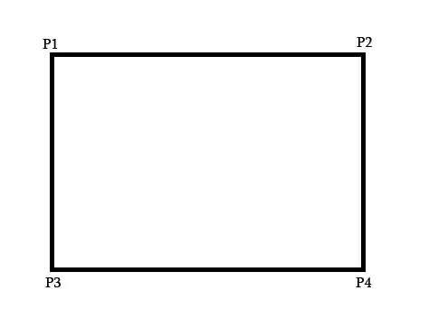
Hence, each pair of points $p_i^{\prime} = \begin{bmatrix}u_i\\ v_i\\ 1\end{bmatrix}, p_i = \begin{bmatrix}x_i\\ y_i\\ 1\end{bmatrix}$, we get $2$ equations.

From $4$ pair of points we get linear system with $2\times 4 = 8$ equations, for $8$ unknowns $h_1,h_2,\ldots,h_8$.

Projective Transform (Homography) having $8$ degrees of freedom, $h_9$ is known or can be obtained from the unknown coefficients, so we have to solve for $8$ unknowns.

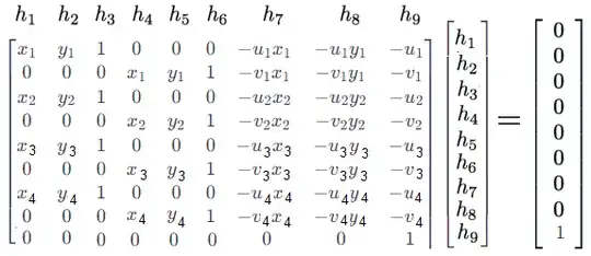
If we assume $h_9=1$, then we have the following linear system of equation ($A\boldsymbol{h}=\boldsymbol{b}$) to solve:

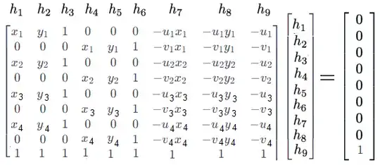
If we assume $\sum\limits_{i=1}^{9}h_i=1$, then we have the following linear system of equation

Assuming $A$ is full-rank, the system has a unique solution and can be obtained as $\boldsymbol{h}=A^{-1}\boldsymbol{b}$, or, more generally, as $\boldsymbol{h}=A^{\dagger}\boldsymbol{b}$, using the Moore-Penrose Pseudoinverse.

Now, let's demonstrate with python:

import numpy as np
import matplotlib.pylab as plt
src = np.array([[14,28],
               [288,28],
                [14,218],
               [288,218]])
dst = np.array([[34,207],
               [281,130],
                [16,29],
               [263,25]])
x, y, u, v = src[:,0], src[:,1], dst[:,0], dst[:,1]
A = np.zeros((9,9))
j = 0
for i in range(4):
    A[j,:] = np.array([-x[i], -y[i], -1, 0, 0, 0, x[i]u[i], y[i]u[i], u[i]])
    A[j+1,:] = np.array([0, 0, 0, -x[i], -y[i], -1, x[i]v[i], y[i]v[i], v[i]])
    j += 2
A[8, 8] = 1   # assuming h_9 = 1
b = [0]*8 + [1]
H = np.reshape(np.linalg.solve(A, b), (3,3))
print(H)
[[  1.68471   ,  -0.09453488,  14.58392177],
[  0.05006887,  -0.97074686, 242.75163122],
   [  0.00264368,   0.00027783,   1.        ]]
ps, p1s = [], []
for i in range(4):
    p, q = src[i], dst[i]
    p_hom = [p[0], p[1],1] 
    p1_hom = H@p_hom
    p1 = [x / p1_hom[2] for x in p1_hom[:-1]]
    ps.append(p)
    p1s.append(p1)
    print("P:{}, P':{}, H@P:{}".format(p, q, p1))
P:[14 28], P':[ 34 207], H@P:[34.0, 207.00000000000003]
P:[288  28], P':[281 130], H@P:[281.0, 130.0]
P:[ 14 218], P':[16 29], H@P:[16.0, 29.0]
P:[288 218], P':[263  25], H@P:[263.0, 24.999999999999986]
plot the original and transformed points
ps, p1s = np.array(ps), np.array(p1s)
max_y = 300
plt.figure(figsize=(10,3))
plt.subplot(121),   plt.scatter(ps[:,0], max_y-ps[:,1], color='g', s=50), plt.title('P', size=20), plt.grid()
plt.subplot(122),   plt.scatter(p1s[:,0], max_y-p1s[:,1], color='r', s=50), plt.title(r'P$^{\prime}$', size=20), plt.grid()
plt.show()

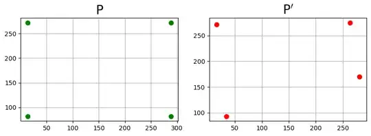
As can be seen, the transformed coordinates are same as the ground-truth ones (upto numerical precision) with the estimated homography matrix.

Reference: https://www.cs.cmu.edu/~16385/lectures/lecture9.pdf