Wiggly polynomials

Question

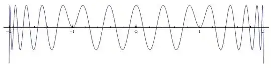
I'd like to be able to construct polynomials $p$ whose graphs look like this:

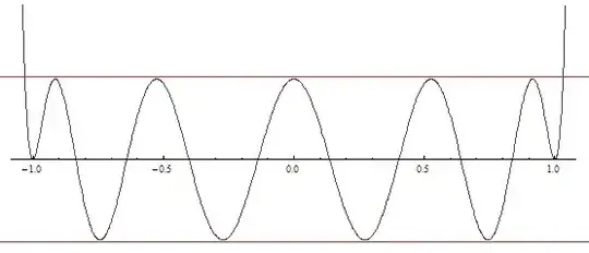
We can assume that the interval of interest is $[-1, 1]$. The requirements on $p$ are:

(1) Equi-oscillation (or roughly equal, anyway) between two extremes. A variation of 10% or so in the values of the extrema would be OK.

(2) Zero values and derivatives at the ends of the interval, i.e. $p(-1) = p(1) =p'(-1) = p'(1) = 0$

I want to do this for degrees up to around 30 or so. Just even degrees would be OK.

If it helps, these things are a bit like Chebyshev polynomials (but different at the ends).

The one in the picture has equation $0.00086992073067855669451 - 0.056750328789339152999 t^2 + 0.60002383910750621904 t^4 - 2.3217878459074773378 t^6 + 4.0661558859963998471 t^8 - 3.288511471137768132 t^{10} + t^{12}$

I got this through brute-force numerical methods (solving a system of non-linear equations, after first doing a lot of work to find good starting points for iteration). I'm looking for an approach that's more intelligent and easier to implement in code.

Here is one idea that might work. Suppose we want a polynomial of degree $n$. Start with the Chebyshev polynomial $T_{n-2}(x)$. Let $Q(x) = T_{n-2}(sx)$, where the scale factor $s$ is chosen so that $Q(-1) = Q(1) = 0$. Then let $R(x) = (1-x^2)Q(x)$. This satisfies all the requirements except that its oscillations are too uneven -- they're very small near $\pm1$ and too large near zero. Redistribute the roots of $R$ a bit (somehow??) to level out the oscillations.

Comments on answers

Using the technique suggested by achille hui in an answer below, we can very easily construct a polynomial with the desired shape. Here is one:

The only problem is that I was hoping for a polynomial of degree 12, and this one has degree 30.

Also, I was expecting the solution to grow monotonically outside the interval $[-1,1]$, and this one doesn't, as you can see here:

Answer 1

Starting with any Chebyshev polynomial of $1^{st}$ kind $T_n(x), n > 2$, and any positive root $a$ of it. Compose $T_n(ax)$ with any polynomial $q(x)$ which is monotonic over $[-1,1]$ that satisfies $q(-1) = -1, q(1) = 1$ and $q'(-1) = q'(1) = 0$ , then $T_n(a q(x))$ is something you want. For example, $$ T_n\left(\cos\left(\frac{\pi}{2n}\right) \frac{x(3-x^2)}{2}\right) $$

Answer 2

Here the Newton version of the Asymptote code that does the job. Now it runs really fast in the range requested. The polynomial is encoded by its roots (stored in the x array). Thanks to the kind soul who had the patience to type 4 spaces in the beginning of each line :).

Edit. Since bubba wanted to know where the main iteration step came from, here is a short explanation. First of all, as I said, it is convenient to work with the sum $f(x)=\sum_k\log|x-x_k|$ instead of the product $\prod_k (x-x_k)$ (for both numerical and analytic reasons). This sum dives to $-\infty$ at each root $x_k$ and achieves a local maxima $y_{k-1}$ and $y_k$ at some points $z_{k-1}\in(x_{k-1},x_k)$ and $z_k\in(x_k,x_{k+1})$. Now, let's make a leap of faith and assume that $y_{k-1}$ and $y_k$ are not very different and also that the $z$-points are approximately in the middle of the corresponding intervals (the first assumption is bound to happen sooner or later if our algorithm works at all and the second one is actually poorly justified by itself but more reasonable than any other wild guess about the location). We want to shift the root $x_k$ so that the maxima $y_{k-1}$ and $y_k$ will become equal. Linearizing and assuming that the intervals $(x_{k-1},x_k)$ and $(x_k,x_{k+1})$ are of approximately equal length, we see that the partial derivatives of $f(z_{k-1})$ and $f(z_k)$ with respect to $x_k$ are about $\frac{1}{4(x_{k+1}-x_{k-1})}$ and $-\frac{1}{4(x_{k+1}-x_{k-1})}$ respectively, so, solving the corresponding linear equation, we get the correction $p=(y_k-y_{k-1})(x_{k+1}-x_{k-1})/8$ to apply to $x_k$. That explains the main formula. Unfortunately, if we just use it literally, a lot of crazy things may happen up to the loss of the order of roots, so we should make sure that our shifts are not too large at the early stages when the disbalances are quite large. The second line is a mere truncation of the shifts to the size which, we believe, will constitute only a fraction of the distance between roots (which initially is $2/n$), so that no rearrangement of roots or screwing up of the Newton iteration scheme will occur. The exact choice of the constant $0.3$ is empirical (i.e., I just checked that it worked in the requested range and, say, $0.5$ did not). The formal justification of the algorithm will require quite a lot of careful estimates (you can easily notice that some of the assumptions I made are on the border of wishful thinking) but, since all we need is one sequence of polynomials of not too high degree, I thought it would be worth trying without worrying too much about formal proofs because the final result is verifiable and once you get it, who cares what steps led to it? I know, this is a dismal thing to say for a mathematician, but, since I'm wearing a programmer's hat here, I decided I could try to get away with it :).

int n=51;
//The number of intermediate roots plus 1 (degree-3)

real[] x,y,z;
//The root array, the maximum array. and the critical point array

for(int k=0;k<n+1;++k) {x[k]=2*k/n-1; if(k>0) z[k-1]=(x[k-1]+x[k])/2;} 
//Just initialized the roots to an arithmetic progression
//and the critical points to midpoints between roots

real f(real t)
{
real s=2*log(1-t^2);
for(int k=1;k<n;++k) s+=log(abs(t-x[k]));
return s;
}
//This is just the logarithm of the absolute value of the polynomial
//with double roots at +1,-1 and simple roots at x[k], k=1,...,n-1

real g(real t)
{
real s=2*(1/(t+1)+1/(t-1));
for(int k=1;k<n;++k) 
s+=1/(t-x[k]);
return s;
}
//This is the derivative of f

real G(real t)
{
real s=-2*(1/(t+1)^2+1/(t-1)^2);
for(int k=1;k<n;++k) 
s-=1/(t-x[k])^2;
return s;
}
//This is the derivative of g

for(int m=0;m<15*n+30;++m)
//The outer cycle; the number of iterations is sufficient 
//to cover n up to 70 with the roots found with machine precision (1E-15) 
{
  for(int k=0;k<n/2;++k) 
  {
    real a=z[k];
    a-=g(a)/G(a); 
    y[k]=f(a); y[n-1-k]=y[k];
    z[k]=a; z[n-1-k]=-a;
  }
  //Newton update of critical points with symmetry taken into account

  real[] xx=copy(x);
  for (int k=1;k<n/2;++k) 
  { 
    real p=(y[k]-y[k-1])*(xx[k+1]-xx[k-1])/8; 
    if (abs(p)>0.3/n) p*=0.3/n/abs(p);
    x[k]+=p; x[n-k]-=p;   
  }
//The main iteration step: move each roots to balance the maxima
//adjacent to it. It can be done 
//better if we look beyond the adjacent maxima to evaluate what will 
//happen but, since it works in a reasonable time, I was too lazy to bother.

}

write(x);
write(y);
//outputs the roots and the maxima of f. Note that the roots at +1 and -1
//are double and the rest are simple.

pause();
//Just doesn't let the window close before you look at it.