Solving for constant of a known nonlinear dynamic system, numerically

Question

Given a dynamic system, \begin{equation*} \frac{d\vec{s}}{dt}=f(t,\vec{s},\vec{c}) \end{equation*} where $\vec{s}$ are the state, and $\vec{c}$ are constants.

And $\vec{s_0},\vec{s_1},...\vec{s_n}$ for $t_0,t_1,...t_n$, assume $n>>$ dimension of $\vec{s}$ and $\vec{c}$

1. How do find $\vec{c}$ numerically?
2. Is it even possible?

---

---

I assume you can just use least_square to solve for those constants since the number of sample data point is way bigger than than the number of constant needed to be solve.

To test that, I solve for the ivp of the system and try to apply least square but it doesn't works

for a simple example, $\vec{s}=[\theta\quad\omega]^T$

\begin{align*} \frac{d\theta}{dt} &= \omega\\ \frac{d\omega}{dt} &= C_0[\sin(t)-\theta] \end{align*}

to model it with python

import numpy
def construct_state_space_eq(C_0):
def state_space_eq(t,x):
    return [
        x[1],
        C_0 * (np.sin(t)-x[0])
    ]

return state_space_eq

and solve the ivp

import scipy
start = 0 
end = 10
sol = scipy.integrate.solve_ivp(
    construct_state_space_eq(100),
    [start,end],
    [0,0],
    max_step=0.001
)

and to retrieve data from solution

time = sol.t
angle = sol.y[0]
speed = sol.y[1]
accel = np.diff(angle)/np.diff(time)
accel = np.array([*accel,accel[-1]])

and then define the error to minimize

def dyn(x):
    C_0, = x
    lhs = np.array([speed, accel])
    rhs = construct_state_space_eq(C_0)(time,[angle,speed])
    return np.sum(np.square(lhs - rhs),axis=0)

and try to minimize the error

guess = [100] # the actual C_0
sol = scipy.optimize.least_squares(
    dyn,
    guess,
    bounds=[0,1000]
)
print(sol.x) # array([0.22989073]) <= but it should be 100

but the result is way off, no matter what the initial guess is.

Is there something fundamentally wrong with my assumption?

Answer 1

Assuming unknown $C_0$ as well as the initial conditions $c_1,c_2$. Solving the ode system we arrive at

$$ \left\{ \begin{array}{l} \theta(t,\Phi)= \frac{c_1 \sin \left(\sqrt{C_0} t\right)}{\sqrt{C_0}}+c_2 \cos \left(\sqrt{C_0} t\right)+\frac{C_0 \sin (t)}{C_0-1} \\ \omega(t,\Phi)= c_1 \cos \left(\sqrt{C_0} t\right)-\sqrt{C_0} c_2 \sin \left(\sqrt{C_0} t\right)+\frac{C_0 \cos (t)}{C_0-1} \\ \end{array} \right. $$

where $\Phi=\{C_0,c_1,c_2\}$. Having data $\{\theta_k,\omega_k\}$ we can establish a deviation measure as

$$ \delta_k(\Phi) = \cases{\theta(t_k,\Phi)-\theta_k\\ \omega(t_k,\Phi)-\omega_k} $$

and also a sum of deviations squared

$$ D(\Phi) = \sum_{k=0}^n\|\delta_k(\Phi)\|^2 $$

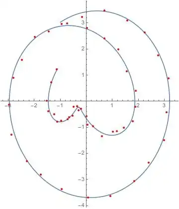
the determination of $\Phi$ can be done using a minimization procedure. Follows a MATHEMATICA script showing all steps.

{thetat, omegat} = {theta[t], omega[t]} /. DSolve[{theta'[t] == omega[t], omega'[t] == c0 (Sin[t] - theta[t])}, {theta, omega}, t][[1]] /. {C[1] -> c1, C[2] -> c2};
(*** DATA PREPARATION ***)
{thetat0, omegat0} = {thetat, omegat} /. {c0 -> 2, c1 -> 1, c2 -> -1};
mu1 = 0.1;
mu2 = 0.15;
tmax = 4 Pi;
n = 50;
delta = tmax/n;
data = Table[{thetat0 + RandomReal[mu1 {-1, 1}], omegat0 + RandomReal[mu2 {-1, 1}]}, {t, 0, tmax, delta}];
(*** MINIMIZATION PROCEDURE ***)
res[k_] := {thetat, omegat} /. {t -> delta (k - 1)}
obj = Sum[(res[k] - data[[k]]).(res[k] - data[[k]]), {k, 1, Length[data]}];
sol = NMinimize[{obj, c0 > 0}, {c0, c1, c2}]
{thetatf, omegatf} = {thetat, omegat} /. sol[[2]];
grf = ParametricPlot[{thetatf, omegatf}, {t, 0, tmax}];
grd = ListPlot[data, PlotStyle -> Red];
Show[grf, grd]

Follows a plot showing in red the data points and in blue the parametric plot for $(\theta(t,\Phi_0),\omega(t,\Phi_0))$ after $\Phi_0$ determination. The values found for $\Phi$ are quite accurate considering the data determination used values.

NOTE

In the general case, when $\dot x = f(x,\Phi)$ can't be integrated to a closed form, we can proceed as in this post.