72

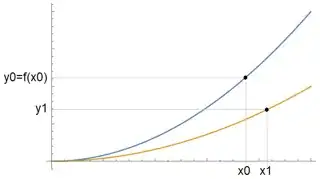
Consider the function $f(x)=a_0x^2$ for some $a_0\in \mathbb{R}^+$. Take $x_0\in\mathbb{R}^+$ so that the arc length $L$ between $(0,0)$ and $(x_0,f(x_0))$ is fixed. Given a different arbitrary $a_1$, how does one find the point $(x_1,y_1)$ so that the arc length is the same?

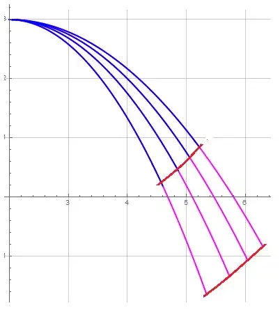
Schematically,

enter image description here

In other words, I'm looking for a function $g:\mathbb{R}^3\to\mathbb{R}$, $g(a_0,a_1,x_0)$, that takes an initial fixed quadratic coefficient $a_0$ and point and returns the corresponding point after "straightening" via the new coefficient $a_1$, keeping the arc length with respect to $(0,0)$. Note that the $y$ coordinates are simply given by $y_0=f(x_0)$ and $y_1=a_1x_1^2$. Any ideas?

My approach: Knowing that the arc length is given by $$ L=\int_0^{x_0}\sqrt{1+(f'(x))^2}\,dx=\int_0^{x_0}\sqrt{1+(2a_0x)^2}\,dx $$ we can use the conservation of $L$ to write $$ \int_0^{x_0}\sqrt{1+(2a_0x)^2}\,dx=\int_0^{x_1}\sqrt{1+(2a_1x)^2}\,dx $$ which we solve for $x_1$. This works, but it is not very fast computationally and can only be done numerically (I think), since $$ \int_0^{x_1}\sqrt{1+(2a_1x)^2}\,dx=\frac{1}{4a_1}\left(2a_1x_1\sqrt{1+(2a_1x_1)^2}+\operatorname{arcsinh}{(2a_1x_1)}\right) $$ Any ideas on how to do this more efficiently? Perhaps using the tangent lines of the parabola?

More generally, for fixed arc lengths, I guess my question really is what are the expressions of the following red curves for fixed arc lengths:

enter image description here

Furthermore, could this be determined for any $f$?

Edit: Interestingly enough, I found this clip from 3Blue1Brown. The origin point isn't fixed as in my case, but I wonder how the animation was made (couldn't find the original video, only a clip, but here's the link)

enter image description here

For any Mathematica enthusiasts out there, a computational implementation of the straightening effect is also being discussed here, with some applications.

mr_e_man
  • 5,986
sam wolfe
  • 3,465
  • 10
    It seems to me that the red curves are orthogonal to the blue curves; that means that you could find an equation for the slope of the red curve at any given point via the slope of the corresponding blue curve, which would give a (hopefully tractable) differential equation to solve for the red curve. – Greg Martin Jul 28 '21 at 17:57
  • @GregMartin this seems like an interesting idea, but I need a bit more details on this. How could we build the differential equation? – sam wolfe Jul 28 '21 at 19:45
  • @samwolfe I have built the differential equation below, but I have not been able to solve it – Ninad Munshi Jul 28 '21 at 19:50
  • @NinadMunshi Thanks, I will take a look. I wonder why this is tricky. If $f(x)=ax$, for example, these red curves are simply circles of radius $L$. – sam wolfe Jul 28 '21 at 20:15
  • 2
    The innermost red curve on the blue and red graphic doesn't look right. It seems to me its topmost point should be somewhat lower down along the leftmost parabola. – Barry Cipra Jul 28 '21 at 20:29
  • @BarryCipra this was made by hand, just as a sketch of what to expect. They are definitely not correct. – sam wolfe Jul 28 '21 at 20:30
  • 2
    @samwolfe, ah good, so my eye (perhaps) did not deceive me. – Barry Cipra Jul 28 '21 at 20:31
  • I like the idea of orthogonal curves, but how do we prove they actually are orthogonal? – Тyma Gaidash Jul 29 '21 at 14:26
  • 1
    @TymaGaidash maybe if you assume they aren't orthogonal you can show that the arc length cannot be preserved. This is the image I keep in mind: https://i.sstatic.net/Q7dG3.png Ultimately we're just tracking the intersection points of those red lines with the parabola, I guess. As if bending/flattening a 2D nail board. – sam wolfe Jul 29 '21 at 14:31
  • @samwolfe you can prove they are in fact not orthogonal because if they were, the dot product of the gradient of $g(x,y)=\frac{y}{x^2}$ with the gradient below would be zero. – Ninad Munshi Jul 29 '21 at 15:42
  • 1
    The orthogonal curves to a parabola are ellipses as seen in this tutor video. – Тyma Gaidash Jul 29 '21 at 16:16
  • @samwolfe you may be able to find the source code for that video here https://github.com/3b1b/videos. edit: this might be it. There's a "PullCurveStraight" function. https://github.com/3b1b/videos/blob/33609fb7b0fd2af834fb764116a3fec662a1d762/so_old_as_to_ignore/homeless.py – mowwwalker Jul 29 '21 at 17:09
  • +1. Very nice question. In theory, the arc length function is invertible but its inverse may be hard to compute. I tried similar problems ("find the points on the curve that divides it equally") and computations are often complicated. – Taladris Jul 30 '21 at 05:49
  • 1
    The endpoints in the animation seem to move in straight (diagonal) lines, so I don't think its creators were aiming at anything meaningful. – Ruslan Jul 30 '21 at 12:05
  • @Ruslan yes, I believe this animation is not reliable. For an approach at recreating the animation with preserved arc lengths, check the linked question on Mathematica's StackExchange (at the bottom of this question). – sam wolfe Jul 30 '21 at 12:15
  • 2
    "Determining the length of an irregular arc segment is also called rectification of a curve" (Wikipedia). So the word "straighten" you use is related to a more formal word rectify that is used when calculating (in any way) arc lengths. – Jeppe Stig Nielsen Jul 30 '21 at 15:08
  • 1
  • Great question! Perhaps it's also interesting to consider a generalization of this question: how to straighten functions of the form $f(x) = a x^{2n} $ for any positive integer $n$ ? – Max Lonysa Muller Jul 03 '23 at 08:37

7 Answers7

33

Phrased differently, what we want are the level curves of the function

$$\frac{1}{2}f(x,y) = \int_0^x\sqrt{1+\frac{4y^2t^2}{x^4}}\:dt = \frac{1}{2}\int_0^2 \sqrt{x^2+y^2t^2}\:dt$$

which will always be perpendicular to the gradient at that point

$$\nabla f = \int_0^2 dt\left(\frac{x}{\sqrt{x^2+y^2t^2}},\frac{yt^2}{\sqrt{x^2+y^2t^2}}\right)$$

Now is the time to naturally reintroduce $a$ as the parameter for these curves. Therefore what we want is to solve the differential equation

$$x'(a) = \int_0^2 \frac{-axt^2}{\sqrt{1+a^2x^2t^2}}dt \hspace{20 pt} x(0) = L$$

where we substitute $y(a) = a\cdot x^2(a)$, thus solving for one component automatically gives us the other.


EDIT: Further investigation has led me to some interesting conclusions. It seems like if $y=f_a(x)$ is a family strictly monotonically increasing continuous functions and $$\lim_{a\to0^+}f_a(x) = \lim_{a\to\infty}f_a^{-1}(y) = 0$$

Then the curves of constant arclength will start and end at the points $(0,L)$ and $(L,0)$. Take for example the similar looking family of curves

$$y = \frac{\cosh(ax)-1}{a}\implies L = \frac{\sinh(ax)}{a}$$

The curves of constant arclength are of the form

$$\vec{r}(a) = \left(\frac{\sinh^{-1}(aL)}{a},\frac{\sqrt{1+a^2L^2}-1}{a}\right)$$

Below is a (sideways) plot of the curve of arclength $L=1$ (along with the family of curves evaluated at $a=\frac{1}{2},1,2,4,$ and $10$), which has an explicit equation of the form

$$x = \frac{\tanh^{-1}y}{y}\cdot(1-y^2)$$ enter image description here

These curves and the original family of parabolas in question both have this property, as well as the perfect circles obtained from the family $f_a(x) = ax$. The reason the original question was hard to tractably solve was because of the non analytically invertible arclength formula

Ninad Munshi
  • 37,891
  • The brown, blue parabolas in the plot seem to have lengths more than $ L= 1$. – Narasimham Jul 31 '21 at 21:07
  • @Narasimham they are not parabolas, nor is the scale on these plots 1:1. I tried my best to play around with the plot options but the progeam likes to automatically break the visual consistency – Ninad Munshi Jul 31 '21 at 22:13
  • This is quite an astonishing approach. How did you come up with those parabola-like curves? Interesting that the parabola case is hard to solve, but I guess in the end it will always rely on how difficult the arclength equation is, like you said. In Mathematica we can get pretty good approximations (see linked question). – sam wolfe Jul 31 '21 at 22:54
  • Should n't the bent/straightened curves be also parabolas? – Narasimham Aug 01 '21 at 19:58
  • @Narasimham I think you should read my post to figure out what is going on. This is a family of hyperbolic cosines. I wanted to give an example that wasn't computationally expensive so I found similar looking curves that had analytically invertible arc lengths. – Ninad Munshi Aug 01 '21 at 20:53
  • 1
    @samwolfe thank you, I appreciate it. I just tried to make use of anything where $\sqrt{1+f^2}$ simplified nicely. This only leaves a few analytic options, such as $\sinh(ax)$ and $\tan(ax)$. From there, choose the antiderivative that contains $(0,0)$ for all $a$. – Ninad Munshi Aug 01 '21 at 20:56
  • 1
    @samwolfe I think that an interesting problem would be going the reverse way - if we had a curve that connects $(0,L)$ to $(L,0)$, could we find a family of curves for which they are a constant arc length away from the origin for? For example, how could one get $ax$ from the equation $x^2+y^2=L^2$ ? or any other curve for that matter – Ninad Munshi Aug 01 '21 at 21:02
  • Thanks. My question was to OP sam wolfe about his question. – Narasimham Aug 02 '21 at 07:35
  • @NinadMunshi that's probably an even better question. Even just thinking of polynomial functions $f(x)=a_0+a_1x+a_2x^2+\cdots +a_nx^n$, one could ask for which parameter region would make $L(a_0,a_1,a_2,...,a_n)$ "invertible" enough so that $x^2+y^2=L^2$ is analytically solvable. Is there even an invertible solution of $n>1$? Interesting that polynomials are tricky for this problem. I really like your approach because from a data fitting perspective, I could avoid the parabolic flattening by fitting my data points with a more analytically suitable function such as those. – sam wolfe Aug 02 '21 at 13:03
  • @NinadMunshi apologies for going back to this question almost one year later, but could you please clarify the definition of function $f(x,y)$ and the change to the integral in the interval $[0,2]$? I must be missing a step. – sam wolfe Jul 16 '22 at 14:20
  • I don't know how useful a tip this may be, but you can set the option AspectRatio->1 for your plot (the default is 1/GoldenRatio I believe), then adjust the PlotRange as needed. – user170231 Dec 19 '22 at 18:11
  • 1
    @samwolfe no worries! I used the substitution $t \mapsto \frac{2t}{x}$ which changes the bounds from $\frac{2(0)}{x} = 0$ to $\frac{2(x)}{x} = 2$ – Ninad Munshi Jun 30 '23 at 20:42
  • @user170231 that did work! The plots I was able to make look so much nicer. Thank you. I may not update the post with plots however unless you would really like me to. – Ninad Munshi Jun 30 '23 at 20:46
23

$L$ being the known arc length, let $x_1=\frac t{2a}$ and $k=4a_1L$; then you need to solve for $t$ the equation $$k=t\sqrt{t^2+1} +\sinh ^{-1}(t)$$A good approximation is given by $t_0=\sqrt k$.

Now, using a Taylor series around $t=t_0$ and then series reversion gives $$t_1=\sqrt{k}+z-\frac{\sqrt{k} }{2 (k+1)}z^2+\frac{(3 k-1) }{6 (k+1)^2}z^3+\frac{(13-15 k) \sqrt{k} }{24 (k+1)^3}z^4+\cdots$$ where $$z=-\frac{\sqrt{k(k+1)} +\sinh ^{-1}\left(\sqrt{k}\right)-k}{2 \sqrt{k+1}}$$

Let us try for $k=10^n$ $$\left( \begin{array}{ccc} n & \text{estimate} & \text{solution} \\ 0 & 0.4810185 & 0.4819447 \\ 1 & 2.7868504 & 2.7868171 \\ 2 & 9.8244940 & 9.8244940 \\ 3 & 31.549250 & 31.549250 \\ 4 & 99.971006 & 99.971006 \\ 5 & 316.21678 & 316.21678 \\ 6 & 999.99595 & 999.99595 \end{array} \right)$$ This seems to be quite decent.

14

Complex Integral

We use the inverse Laplace transform. Define $f(x)=\int_0^x\sqrt{t^2+1}dt=\frac12x\sqrt{x^2+1}+\frac12\sinh^{-1}(x)$ and $g(x)=f^{-1}(x)$. $g(x)’s$ Laplace transform is:

$$\operatorname L_s(g(x))=\int_0^\infty e^{-st}g(t)dt=\int_0^\infty te^{-sf(t)}f’(t)dt$$

where $t\to f(t)$ was substituted. Next, one can integrate by parts and substitute $t\to\sinh(\frac t2)$ to get:

$$\operatorname L_s(g(x))=\frac1s\int_0^\infty e^{-sf(t)}dt=\frac1{2s}\int_0^\infty\cosh\left(\frac t2\right)e^{-\frac s4(\sinh(t)+t)}dt=\frac1{4s}\int_0^\infty e^{-\left(\frac s4-\frac12\right)t -\frac s4\sinh(t)}+e^{-\left(\frac s4+\frac12\right)t -\frac s4\sinh(t)}dt$$

which is the associated Anger Weber function. Applying the inverse Laplace transform gives the inverse function. Therefore:

$$f(x)=\frac12x\sqrt{x^2+1}+\frac12\sinh^{-1}(x)\implies f^{-1}(x)=\int_{c-i\infty}^{c+i\infty}\frac{e^{4sx}}{8is}\left(\operatorname A_{s-\frac12}(s)+\operatorname A_{s+\frac12}(s)\right)ds$$

which seems to work for all $x\in\Bbb R$.

enter image description here

Series Solution near $x=0$

If $f(x)=\int_0^x\sqrt{t^2+1}dt$ and $y=f^{-1}(x)$, then one notices: $$3Yy’-y^2=1,Y=\int_0^xy(t)dt$$

Software series reversion shows $x\approx y=\sum\limits_{n=0}^\infty a_nx^{2n+1}$ near $x=0$:

$$3\sum_{k=0}^\infty a_k (2k+1)x^{2k}\sum_{m=0}^\infty\frac{a_mx^{2m+2}}{2m+2}-\sum_{k=0}^\infty a_kx^{2k+1}\sum_{m=0}^\infty a_m x^{2m+1}=1$$ gathering powers of $x$ and simplifying gives:

$$\begin{align}f(x)=\frac12x\sqrt{x^2+1}+\frac12\sinh^{-1}(x)\\\implies f^{-1}(x)=\sum_{n=0}^\infty a_n(-1)^nx^{2n+1}\\a_n=\sum_{m=0}^{n-1}a_ma_{n-m-1}\left(\frac3{2m+2}-\frac4{2n+1}\right)\\=\left\{1,\frac16,\frac{13}{120},\frac{493}{5040},\frac{37369}{362880},\frac{4732249}{39916800},\dots\right\}\end{align}$$

The denominators are $(2n+1)!$, but the numerators do not have an explicit form yet. The series works for $x\in\Bbb C$ too. Here is a plot for $n=11$:

General Series Solution

Unfortunately, the above series has a small convergence radius, so one can use @Paul Enta’s method here to expand $y=f^{-1}(x)$ near $x=x_0$. One notices the polynomial $P_n(x)$:

$$\frac{d^ny}{dx^n}=\frac{P_n(y)}{(y^2+1)^{\frac{3n}2-1}}\iff P_{n+1}=(y^2+1)^\frac{3n+1}2\frac{d^{n+1}y}{dx^{n+1}}= (y^2+1)^\frac{3n+1}2\frac{dy}{dx}\frac d{dy}\left(\frac{d^ny}{dx^n}\right)$$

This finally gives:

$$\begin{align}f(x)=\frac12x\sqrt{x^2+1}+\frac12\sinh^{-1}(x)\\\implies y=f^{-1}(x)=y(x_0)+\sum_{n=1}^\infty\frac{P_n(y(x_0))(x-x_0)^n}{(y^2(x_0)+1)^{\frac{3n}2-1}n!}\\P_{n+1}(x)=(x^2+1)P’_n(x)+(2-3n)xP_n(x)\\=\{1,-x,3x^2-1,13x-15x^3,105x^4-162x^2+13,-493x+2202x^3-945x^5,10395x^6-33351x^4+14001x^2-493,\dots\}\end{align}$$

At $x=0$, this reduces to $P_{n+1}(0)=P’_n(0)$

Mathematica Function

Because of the domain of Mathematica’s Inverse Beta Regularized $\text I^{-1}_s(a,b)$, it solves:

$$\text{ArcLength}(x^2)=\frac12\sqrt{4x^2+1}+\frac14\sinh^{-1}(2x)=z\in\Bbb I\text{ pure imaginary}\implies x\mathop=^{|\text{Im}(z)|\le \frac{\pi}8}\mp\frac i2\sqrt{\text I^{-1}_\frac{\pm8i z}\pi\left(\frac12,\frac32\right)}$$

Plot of $k\in\Bbb R$ vs $\mp\frac i2\sqrt{\text I^{-1}_\frac{\pm8i z}\pi\left(\frac12,\frac32\right)},z=ik$ where opposite signs are taken:

enter image description here

as shown here for $k\in\Bbb R$. The power series in Quantile mechanics, however, extends the domain to complex, and therefore real values. Another expansion there can be found in terms of the Student quantile as it is a special case of $\text I^{-1}_x\left(\frac12,\frac32\right)$


@Francisco Alvarado found an integral solution here. Additionally, previous revisions of this answer have older fixed point iteration solutions.

Тyma Gaidash
  • 13,576
11

Here's about the most efficient thing I can see is this:

Take your antiderivative (replacing the sin with a sinh) and define $a_1 x \equiv y$ so that

$$f(y) = a_1 * (\textrm{arc length}),$$

$$f(y) \equiv \frac{1}{2}(y \sqrt{1+y^2}+ \sinh^{-1} y).$$

$f(y)$ is monotonic and has some nice approximations when $y \ll 1, y \gg 1$. In those cases it might be possible to obtain it analytically. In general, invert it numerically. Then,

$$x = a_1^{-1} f^{-1}(a_1 * (\textrm{arc length}).$$

The utility of doing it this way is that you don't have to keep inverting a new function for each new $a_1$, you only have to do it once to be able to flatten any parabola you want.

David
  • 1,659
  • 1
    The notation $a\ast b$ often means the convolution of $a$ and $b$. I think it's clear enough from context that is not what you mean, but since the question does seem to naturally involve integrals, it may be clearer to use \cdot instead of * or \ast – Alex Ortiz Jul 31 '21 at 19:29
9

TLDR:

You want to solve for $v$ in this equation: $$v\sqrt{v^2+1} + \sinh^{-1} v = 2a_1x_0\sqrt{u^2+1} + \frac{\sinh^{-1} u}{2a_0}$$

And then $x_1=\frac{v}{2a_1}$ is your solution.

I’ve been banging away at this for hours, not because I think I can help you—much of this is new to me—but because I found it interesting. I haven’t yet worked out (an approximation to a) solution for $v$, though. And it looks like Claude’s answer has beaten me to it, anyway.

But here is my working, just because I can’t bear to hit Discard on this whole thing.


I don’t think I’ve ever done the length of a parabolic curve before. So while this would probably go more smoothly if done from the integral definition of arc length, I’m going to take the easy(?) way out: Wikipedia has a parabolic arc length formula. Let’s give it a go!


So we have a parabola $f\left(x\right)=a_0 x^2$. Wikipedia tells us that we can find the arc length, from the vertex at $\left(0,0\right)$ to any point $\left(x,f\left(x\right)\right)$ on the parabola, using these values:

  • The focal length $l$ of the parabola; in this case, $l=\frac{1}{4a_0}$
  • The perpendicular distance $p$ between the point and the axis of symmetry; in this case it’s simply $p=x$

Then, given $h=\frac{p}{2}$ and $q=\sqrt{l^2+h^2}$, the arc length is:

$$s=\frac{hq}{l}+l\ln\frac{h+q}{l}$$

Let’s simplify. Given that $h=\frac{x}{2}$

$$\begin{align} q &= \sqrt{\frac{1}{16a_0^2}+\frac{x^2}{4}} \\ &= \sqrt{\frac{4a_0^2x^2+1}{16a_0^2}} \\ &= l\sqrt{4a_0^2x^2+1} \end{align}$$

Thus:

$$s=\frac{x}{2}\sqrt{4a_0^2x^2+1}+\frac{1}{4a_0}\ln\left(2a_0x+\sqrt{4a_0^2x^2+1}\right)$$


Now, we have another parabola $g(x)=a_1 x^2$ such that the arc lengths of $f\left(x_0\right)$ and $g\left(x_1\right)$ are equal, i.e.:

$$\begin{align} \frac{x_0}{2}\sqrt{4a_0^2x_0^2+1}+\frac{1}{4a_0}\ln\left(2a_0x_0+\sqrt{4a_0^2x_0^2+1}\right) &= \frac{x_1}{2}\sqrt{4a_1^2x_1^2+1}+\frac{1}{4a_1}\ln\left(2a_1x_1+\sqrt{4a_1^2x_1^2+1}\right) \\ \therefore x_0\sqrt{4a_0^2x_0^2+1}+\frac{1}{2a_0}\ln\left(2a_0x_0+\sqrt{4a_0^2x_0^2+1}\right) &= x_1\sqrt{4a_1^2x_1^2+1}+\frac{1}{2a_1}\ln\left(2a_1x_1+\sqrt{4a_1^2x_1^2+1}\right) \end{align}$$

And we want to solve for $x_1$ in terms of $a_0$, $a_1$, and $x_0$. Nothing simpler! </sarc>


Let’s define $u=2a_0x_0$ (thus $u^2=4a_0^2x_0^2$) and $v=2a_1x_1$ (thus $v^2=4a_1^2x_1^2$). That shortens things to:

$$x_0\sqrt{u^2+1} + \frac{1}{2a_0}\ln\left(u+\sqrt{u^2+1}\right) = x_1\sqrt{v^2+1} + \frac{1}{2a_1}\ln\left(v+\sqrt{v^2+1}\right)$$

Now I see where $\sinh$ comes into the other answers! It’s because $\sinh^{-1} x = \ln\left(x+\sqrt{x^2+1}\right)$, so we get:

$$\begin{align} x_0\sqrt{u^2+1} + \frac{\sinh^{-1} u}{2a_0} &= x_1\sqrt{v^2+1} + \frac{\sinh^{-1} v}{2a_1} \\ \therefore 2a_1x_0\sqrt{u^2+1} + \frac{\sinh^{-1} u}{2a_0} &= 2a_1x_1\sqrt{v^2+1} + \sinh^{-1} v \\ &= v\sqrt{v^2+1} + \sinh^{-1} v \end{align}$$

That right-hand side does not look easy to invert. I admit, I copped out and asked Wolfram Alpha to do it. And of course it tells me, “no result found in terms of standard mathematical functions”. [sigh…]


Based on Tyma Gaidash’s answer, I went looking into the Lagrange inversion theorem. My engineering-oriented education never covered this, but I think I’ve grasped the basics of it. As I understand it, to solve $y=f(x)$ for $x$, we choose some $z$, such that $f(z)$ is defined and $f'(z)\ne 0$.

Let’s shorten the entire left-hand side of the equation to $w$, and define $w=g\left(v\right)=v\sqrt{v^2+1} + \sinh^{-1} v$. First, let’s find the derivative… by cheating and using Wolfram Alpha: $g'(v)=2\sqrt{v^2+1}$.

We need a value $z$ where $g'(z)\ne 0$. Conveniently, this derivative is nowhere zero on the reals, so that’s trivial. I think (but am not sure) that $z$ should approximate $v$, so let’s randomly assume that $x_1\approx 1$ and so $v\approx 2a_1 = z$.

Now, by the inversion theorem, the inverse function $v=g^{-1}\left(w\right)$ is:

$$\begin{align} v &= z+\sum_{n=1}^\infty \left[\frac{\left(w-g\left(z\right)\right)^n}{n!} \lim_{t\to z} \frac{d^{n-1}}{dt^{n-1}}\left(\frac{t-z}{g(t)-g(z)}\right)^n\right] \\ &= z+\left(w-g\left(z\right)\right)\lim_{t\to z}\frac{t-z}{g(t)-g(z)} + \frac{\left(w - g\left(z\right)\right)^2}{2} \lim_{t\to z}\frac{d}{dt} \left(\frac{t-z}{g(t)-g(z)}\right)^2 + \cdots \end{align}$$

Doesn’t that first limit look just like the reciprocal of the derivative? So the second term of the series becomes $\frac{w-g\left(z\right)}{2\sqrt{z^2+1}}$.

And I’ve been working on this for way too long now, so that’s where I’ll stop for the night.
  • 1
    @TymaGaidash: Those are meant to be initial values, not restrictions—like choosing initial values in Newton's method. And I don’t know if that’s even correct! (Claude’s answer doesn’t appear to have anything like that, but it seems to be the same approach.) But yes, the aim is ultimately to have a solution (or at least an approximate one, from the first few terms of the series) for $v$, at which point the simplifications $v$, $w$ etc. can perhaps be dropped. (Or maybe it’ll end up being clearer to leave them in?) – Tim Pederick Jul 30 '21 at 08:53
4

For a parabola with parametrization

$$ x= at,y= a t^2/2 ;\;x^2= 2 a y \;; \text{slope} \;t=\tan \phi; \tag1$$

Differentiate $x^2$, primed wrt arc length

$$ 2 x \cos \phi = 2 a \sin \phi ;\; x= a \tan \phi ;\;x'= \cos \phi= a \sec^2 \phi \;\phi' \tag 2 $$

from which comes the curvature

$$ a \phi'=a \kappa=\cos^3 \phi \tag 3$$

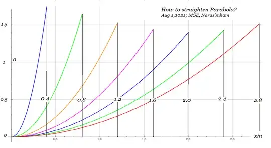
An easier/direct way out is by direct numerical integration of ode in(3). A fraction k of max arc length can be set as a parameter for required integrands ( k= 2/3 in this particular case), making the subset parabolas flatter or deeper by adjusting $a$.

enter image description here

Total length on one side is a given constant $L$

$$ L = \int _0^{\phi_m} \frac{ d \phi}{\kappa} ; \text{ now plug in curvature from(3) and integrate }$$

$$ \frac{L}{a}=\int _0^{\phi_m} \sec^3 \phi\; d\phi = \frac12\bigg[\log\bigg(\tan\bigg(\frac{\pi}{4} + \frac{\phi_m}{2} \bigg)\bigg) +\sec \phi_m \tan \phi_m \bigg]\tag 4 $$

Plug in from (2) $x_{m}=a \tan \phi_m $ $$ \frac{2L}{a}= \log\left(\tan\bigg(\frac{\pi}{4} + \frac{\tan^{-1}(x_m/a)}{2}\right)\bigg)+ (x_m/a) \sqrt{(x_m/a)^2-1} \tag 5 $$

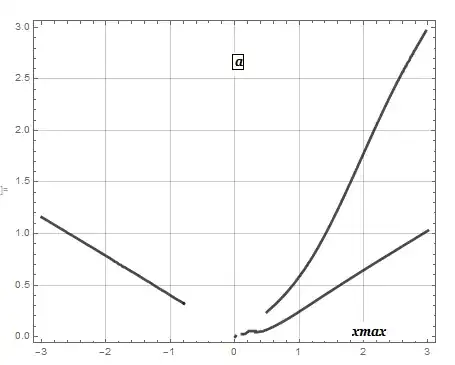
which is a neat implicit function $ f(a,x_m,L) $ , plotted assuming an arm of parabola has given arc length $=1.8,$ on Mathematica, enabling flatter or deeper parabola plots.

enter image description here

It has become clear that there are two criteria for equal parabolic arc lengths connecting $x_{max} $ to $ \text { a = 2* focal-length }$.

EDIT 1/2:

To come out of the apparent dilemma I have carefully calculated/plotted special cases for $( x_{max},a)$ combinations:

$$(0.4,0.0458),(0.8,0.1948), (1.2,0.4704),(1.6,0.8874)(2.0, 1.42264),(2.4,2.0101),(2.8,2.5825)$$

All arcs are all of same length but for $( x_{max} =2.0,2.4,2.8) $ the choice of $a$ seems to have got switched over to the second critirion. Relation $(x_{max},a) $ is not unique by the first plot...it is now examined further.

enter image description here

Narasimham
  • 42,260
1

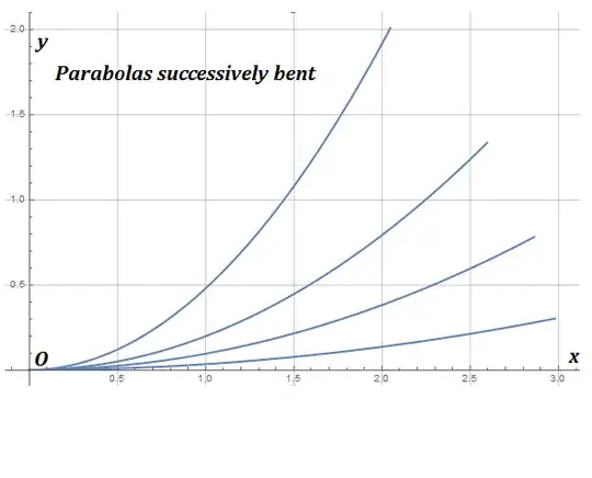
Adding another short ODE method that finds a direct relation between maximum slope at parabola tip and its focal length for invariant arc length while bending.

$$ x = 2 f \tan \phi \;\text {is differentiated w.r.t. arc, } 2f \sec^2\phi \frac{d\phi}{ds}=\cos \phi$$

Integrate back but w.r.t. slope $ \phi, s= 2 f \int \sec^3\phi\; d\phi$

$$ s= 2 f \left(\frac12 \log \frac{\cos (\phi/2)+ \sin (\phi/2) }{\cos (\phi/2)- \sin (\phi/2) } +\sec \phi +\tan \phi \right)= \text{constant}$$

Computed focal length $ f=F(\phi_{max})$ as the relation between bending variables on Mathematicafor maximum slopes $(0.2,0.5,0.8,1.1)$ radians with fixed arc length of parabola 3 units assumed and plotted as shown; $ (x,y)= (2ft,ft^2). $

enter image description here

Narasimham
  • 42,260