Inverse of $x + \sin^2(x)$

Question

I'm looking for the inverse of the function $f(x) = x + \sin^2(x)$. The function is bijective, so the inverse exists.

The graph below shows the function and its inverse.

It appears that the inverse function can be decomposed as $f^{-1}(x)=x+g(x)$. The graph below shows $g(x)$.

Can $g(x)$ be represented using elementary functions or standard special functions?

Answer 1

Applying the double angle formula: $$x+\sin^2(x)=a\iff 2x-\cos(2x)=2a-1$$ Now substitute $2x=w-\frac\pi2$ to get: $$w-\sin(w)=2a-1+\frac\pi2$$ which is a special case of the Kepler equation. This question has methods to solve it. Using its Fourier series solution, we get: $$\boxed{f(x)=x+\sin(x)^2\implies f^{-1}(x)-x=g(x)=-\frac12+\sum_{n=1}^\infty\frac{J_n(n)}n\sin\left(\left(2x-1+\frac\pi2\right)n\right)}$$ as shown here using the Bessel function of the first kind:

---

Other series expansions seem to have double sum recurrence relations, but this answer gives a simpler one to invert $x\sqrt{1-x^2}+\sin^{-1}(x)$: $$\boxed{f(x)=x+\sin(x)^2\implies f^{-1}(x)-x=g(x)=\frac\pi4-x-\sin^{-1}\sum_{n=0}^\infty a_n\left(\frac\pi8+\frac14-\frac x2\right)^{2n+1},\\a_n=\sum_{m=0}^{n-1}a_ma_{n-m-1}\left(\frac3{2m+2}-\frac4{2n+1}\right)\\=\left\{1,\frac16,\frac{13}{120},\frac{493}{5040},\frac{37369}{362880},\frac{4732249}{39916800},\dots\right\}}$$

Answer 2

Don't know if this helps, but if

$$y=x+\sin^2(x) \tag{1}$$

and

$$x=y+g(y) \tag{2}$$

then

$$y=y+g(y)+\sin^2(y+g(y)) \tag{3}$$

and you get an implict equation for $g(y)$:

$$g(y)=-\sin^2(y+g(y)) \tag{4}$$

An iteration scheme such as

$$g_n(y) = -\sin^2(y+g_{n-1}(y)) \tag{5}$$

can be set up, to expose the perodicity of $g$:

$$\begin{cases} g_1(y)=-\sin^2(y) \\ g_2(y)=-\sin^2(y-\sin^2(y)) \\ \cdots \end{cases} \tag{6}$$

We can plot this using Python as follows:

import numpy as np
import matplotlib.pyplot as plt
xs = np.linspace(-np.pi, np.pi, 10**3 + 1)
ys0 = np.zeros_like(xs)
yss = [ys0]
for n in range(20):
    ys_prev = yss[n]
    ys_new = - np.sin(xs + ys_prev)**2
    yss.append(ys_new)
plt.plot(xs, yss[17], color="green", label="g_17")
plt.plot(xs, yss[18], color="red", label="g_18")
plt.plot(xs, yss[19], color="green", label="g_19")
plt.plot(xs, yss[20], color="red", label="g_20")
a = np.linspace(-np.pi, np.pi, 103 + 1)
b = a + np.sin(a)  2
c = b
d = a - b
plt.plot(c, d, color="blue", label="g")
plt.grid()
plt.axhline(color="black")
plt.axvline(color="black")
ax = plt.gca()
ax.set_xlim([-np.pi, np.pi])
ax.set_ylim([-np.pi, np.pi])
ax.set_aspect('equal')
plt.legend(loc="upper left")
plt.xlabel("x")
plt.ylabel("y")
plt.savefig("out.png")
plt.show()

We can see that the $g_n$'s are alternating, with the graph of $g_n$ for even $n$ lying above the graph of $g$ and the graph of $g_n$ for odd $n$ lying below the graph of $g$.

Answer 3

This is not satisfactory.

$$f(x)=x+\sin^2(x)$$ can be quite well represented by a $[2n+1,2n]$ Padé approximant $P_n$ which would write $$f(x) \sim P_n= x \, \frac {1+\sum_{k=1}^{2n} a_n\, x^n } {1+ \sum_{k=1}^{n} b_n\, x^{2n} }$$ The poblem is that this would lead to polynomial equations of very high degree.

To give an idea of the accuracy, consider the norm $$\Phi_n=\int_{-\pi}^{+\pi} \Big(f(x)-P_n\Big)^2\,dx$$ $$\Phi_3=5.32306\times 10^{-3} \qquad \Phi_4= 2.43586\times 10^{-6}\qquad \Phi_5=1.5373\times 10^{-10}$$

For $f(x)=2.345$, $P_4$ would give $x=\color{red}{1.38070249}80$

Answer 4

We can, at the very least, compute the Taylor series of $g(x)$ to a few terms:

We have $$ f(x) = x + \operatorname{sin}(x)^2 \\ = x + \left( x - \frac{1}{6} x^3 + \frac{1}{120} x^5 - \frac{1}{5040} x^7 + \ldots \right)^2 \\ = x + x^2 - \frac{1}{3} x^4 + \frac{2}{45} x^6 - \frac{1}{315} x^8 + \ldots \\ $$

The Lagrange Inversion Formula gives us (using FLINT)

from flint import *
x = fmpq_series([0,1])
print((x + x.sin()**2).reversion())
x + (-1)*x^2 + 2*x^3 + (-14/3)*x^4 + 12*x^5 + (-1472/45)*x^6 + 464/5*x^7 + (-85364/315)*x^8 + 152888/189*x^9 + O(x^10)

$$ f^{-1}(x) = x - x^2 + 2 x^3 - \frac{14}{3} x^4 + 12 x^5 - \frac{1472}{45} x^6 + \frac{464}{5} x^7 - \frac{85364}{315} x^8 + \ldots $$

And hence

$$ g(x) = -x^2 + 2 x^3 - \frac{14}{3} x^4 + 12 x^5 - \frac{1472}{45} x^6 + \frac{464}{5} x^7 - \frac{85364}{315} x^8 + \ldots $$

We can plot this using Python as follows:

import flint
import numpy as np
import matplotlib.pyplot as plt
import matplotlib.ticker as ticker
radius_1 = 0.5
radius_2 = 1.49413
radius_3 = 0.369543
x_series = flint.fmpq_series([0,1])
f_series = x_series + x_series.sin()**2
f_inv_series = f_series.reversion()
g_series = f_inv_series - x_series
def eval_g(x):
    res = 0
    for n in range(g_series.length()):
        coeff_abstract = g_series.coeffs()[n]
        coeff = int(coeff_abstract.p) / int(coeff_abstract.q)
        res += coeff * x**n
    return res
xs = np.linspace(-radius_1, radius_1, 10**3 + 1)
ys = np.vectorize(eval_g)(xs)
plt.plot(xs, ys, color="red", label="h")
a = np.linspace(-radius_2, radius_3, 103 + 1)
b = a + np.sin(a)  2
c = b
d = a - b
plt.plot(c, d, color="blue", label="g")
plt.grid()
plt.axhline(color="black")
plt.axvline(color="black")
ax = plt.gca()
ax.xaxis.set_major_locator(ticker.MultipleLocator(0.2))
ax.yaxis.set_major_locator(ticker.MultipleLocator(0.2))
ax.set_xlim([-radius_1, radius_1])
ax.set_ylim([radius_1 - radius_2, radius_1 - radius_3])
ax.set_aspect('equal')
plt.legend(loc="upper left")
plt.xlabel("x")
plt.ylabel("y")
plt.savefig("out.png")
plt.show()

We can see that beyond the radius of convergence given by $\frac{1}{2} - \frac{\pi}{4}$ (as noted by @JyrkiLahtonen), the Taylor approximation cannot possibly be accurate.

Answer 5

Similar to the answer by @user619894, we can also consider the closely related implicit equation $$ g(y) = \frac{1}{2} \left( - \operatorname{sin}^2(y + g(y)) \right) + \frac{1}{2} g(y) \tag{1a} $$ and the associated iteration scheme $$ g_n(y) = \frac{1}{2} \left( - \operatorname{sin}^2(y + g_{n - 1}(y)) \right) + \frac{1}{2} g_{n - 1}(y) \tag{1b} $$

We can plot this using Python as follows:

import numpy as np
import matplotlib.pyplot as plt
xs = np.linspace(-np.pi, np.pi, 10**3 + 1)
ys0 = np.zeros_like(xs)
yss = [ys0]
for n in range(20):
    ys_prev = yss[n]
    ys_new = (1/2) * (- np.sin(xs + ys_prev)*2) + (1/2)  ys_prev
    yss.append(ys_new)
plt.plot(xs, yss[20], color="red", label="g_20")
a = np.linspace(-np.pi, np.pi, 103 + 1)
b = a + np.sin(a)  2
c = b
d = a - b
plt.plot(c, d, color="blue", label="g")
plt.grid()
plt.axhline(color="black")
plt.axvline(color="black")
ax = plt.gca()
ax.set_xlim([-np.pi, np.pi])
ax.set_ylim([-np.pi, np.pi])
ax.set_aspect('equal')
plt.legend(loc="upper left")
plt.xlabel("x")
plt.ylabel("y")
plt.savefig("out.png")
plt.show()

Or, we can consider the following equation $$ g(y) = - \sqrt{- \operatorname{sin}^2(y + g(y)) \cdot g(y)} \tag{2a} $$ and the associated iteration scheme $$ g_n(y) = - \sqrt{- \operatorname{sin}^2(y + g_{n - 1}(y)) \cdot g_{n - 1}(y)} \tag{2b} $$

We can plot this using Python as follows:

import numpy as np
import matplotlib.pyplot as plt
xs = np.linspace(-np.pi, np.pi, 10**3 + 1)
ys0 = - np.ones_like(xs)
yss = [ys0]
for n in range(20):
    ys_prev = yss[n]
    ys_new = - np.sqrt(- np.sin(xs + ys_prev)*2  ys_prev)
    yss.append(ys_new)
plt.plot(xs, yss[20], color="red", label="g_20")
a = np.linspace(-np.pi, np.pi, 103 + 1)
b = a + np.sin(a)  2
c = b
d = a - b
plt.plot(c, d, color="blue", label="g")
plt.grid()
plt.axhline(color="black")
plt.axvline(color="black")
ax = plt.gca()
ax.set_xlim([-np.pi, np.pi])
ax.set_ylim([-np.pi, np.pi])
ax.set_aspect('equal')
plt.legend(loc="upper left")
plt.xlabel("x")
plt.ylabel("y")
plt.savefig("out.png")
plt.show()

Answer 6

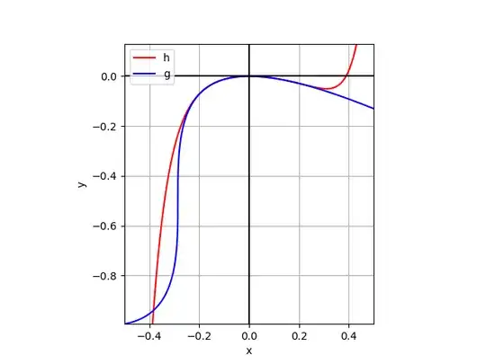
We can also try to use Padé approximants to $g$.

In this first example, we compute Padé approximants $\frac{p_k}{q_k}$ with $\operatorname{deg}(p_k) = \operatorname{deg}(q_k) = k$ such that with $g_k(x) = x^2 \frac{p_k(x)}{q_k(x)}$ we have $g \approx g_k$ ($1 \leq k \leq 3$).

import flint
import numpy as np
import scipy as sp
import matplotlib.pyplot as plt
x_series = flint.fmpq_series([0,1])
f_series = x_series + x_series.sin()2
f_inv_series = f_series.reversion()
g_series = f_inv_series - x_series
h_series_abstract = g_series / x_series2
h_series = [int(coeff_abstract.p) / int(coeff_abstract.q) for coeff_abstract in h_series_abstract.coeffs()]
xs = np.linspace(-np.pi, np.pi, 10**3 + 1)
yss = []
for n in range(1, 3 + 1):
    h_pade_p, h_pade_q = sp.interpolate.pade(h_series, n, n)
    print([h_pade_p, h_pade_q])
    def h_pade(x):
        return x*2  h_pade_p(x) / h_pade_q(x)
    ys = np.vectorize(h_pade)(xs)
    yss.append(ys)
plt.plot(xs, yss[0], color="blue", label="g_1")
plt.plot(xs, yss[1], color="green", label="g_2")
plt.plot(xs, yss[2], color="red", label="g_3")
a = np.linspace(-np.pi, np.pi, 103 + 1)
b = a + np.sin(a)  2
c = b
d = a - b
plt.plot(c, d, color="black", label="g")
plt.grid()
plt.axhline(color="black")
plt.axvline(color="black")
ax = plt.gca()
ax.set_xlim([-np.pi, np.pi])
ax.set_ylim([-np.pi, np.pi])
ax.set_aspect('equal')
plt.legend(loc="upper left")
plt.xlabel("x")
plt.ylabel("y")
plt.savefig("out.png")
plt.show()

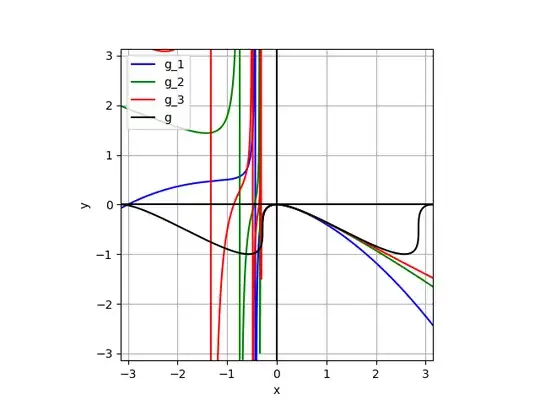
In this second example, we compute Padé approximants $\frac{p_k}{q_k}$ with $\operatorname{deg}(p_k) = \operatorname{deg}(q_k) = k$ such that with $g_k(x) = x \left( \frac{p_k(x)}{q_k(x)} - 1 \right)$ we have $g \approx g_k$ ($1 \leq k \leq 4$).

import flint
import numpy as np
import scipy as sp
import matplotlib.pyplot as plt
x_series = flint.fmpq_series([0,1])
f_series = x_series + x_series.sin()**2
f_inv_series = f_series.reversion()
h_series_abstract = f_inv_series / x_series
h_series = [int(coeff_abstract.p) / int(coeff_abstract.q) for coeff_abstract in h_series_abstract.coeffs()]
xs = np.linspace(-np.pi, np.pi, 10**3 + 1)
yss = []
for n in range(1, 4 + 1):
    h_pade_p, h_pade_q = sp.interpolate.pade(h_series, n, n)
    print([h_pade_p, h_pade_q])
    def h_pade(x):
        return x * (h_pade_p(x) / h_pade_q(x) - 1)
    ys = np.vectorize(h_pade)(xs)
    yss.append(ys)
plt.plot(xs, yss[0], color="blue", label="g_1")
plt.plot(xs, yss[1], color="green", label="g_2")
plt.plot(xs, yss[2], color="red", label="g_3")
plt.plot(xs, yss[3], color="yellow", label="g_4")
a = np.linspace(-np.pi, np.pi, 103 + 1)
b = a + np.sin(a)  2
c = b
d = a - b
plt.plot(c, d, color="black", label="g")
plt.grid()
plt.axhline(color="black")
plt.axvline(color="black")
ax = plt.gca()
ax.set_xlim([-np.pi, np.pi])
ax.set_ylim([-np.pi, np.pi])
ax.set_aspect('equal')
plt.legend(loc="upper left")
plt.xlabel("x")
plt.ylabel("y")
plt.savefig("out.png")
plt.show()

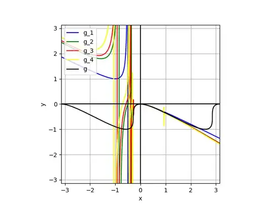
We see that in both cases, the approximations go wild beyond the first vertical slope.