Do you now the domain called Integral Geometry that has other names such as Stochastic Geometry, Geometric measure theory ?
In this framework, a straight line, written under its so-called "polar form":
$$x \cos \theta + y \sin \theta = p,$$
is associated with point $(\theta,p)$ in a "cylindrical space" $H$.
Certain sets of lines will be represented as subsets of $H$ with rather remarkable shapes. Dualy, sine curves in $H$ will be associated to points in the ordinary geometrical space.
For example, being given a point $M$ in the ordinary plane with polar coordinates $(\rho_M, \theta_M)$, the set of lines passing through $A$ is represented in $H$ by the sine curve with equation:
$$\rho=\rho_M \cos(\theta-\theta_M)$$
As a consequence, lines that separate 2 points $A$ and $B$, with resp. polar coordinates $(\rho_A, \theta_A)$ and $(\rho_B, \theta_B)$ (which is equivalent to say that such lines intersect segment $[AB]$) are "positionned" in $H$ in the area between the 2 sine curves with equations:
$$\rho=\rho_A \cos(\theta-\theta_A) \ \ \text{and} \ \ \rho=\rho_B \cos(\theta-\theta_B) \tag{1}$$
Therefore, your problem can be implemented in this space by showing that the set of "points" in $H$ (each point representing a line), defined by a set of $n$ constraints of type (1), is non void.
Some references: an answer of mine here. See also there for the result called "Cauchy-Crofton theorem" allowing to attribute a "degree of margin" one can have in such issues using measure theory.
Remark: The transformation I just described is used under the name "Hough Transform" in image processing.
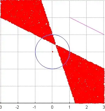
Edit: Here is an apparently different representation using pole polar duality "twining" in a natural way a line to a point, therefore a set of lines to a set of points. In fact this representation is equivalent to the one I have explained before. The big advantage of this representation is that it doesn't need an auxiliary representation space: we always work in the initial space. Technically, it's very simple : to a line with equation $ax+by=1$ is associated its pole $(a,b)$.
Using this correspondence, we can associate to any line segment $[AB]$ the set of lines that intersect it, or more exactly their poles, and the result is simple; the set of lines intersection line segment $[AB]$ is the region situated between the to polar lines of $A$ and $B$ resp. Here is the case (line segment with magenta color). Thousands of random lines intersecting $[AB]$ have been considered and their poles represented by red points materializing the area between the two polar lines of extreme points $A$ and $B$:
Doing this for line segments $[A_kB_k], \ \ k=1,2...N$ gives a constructive testing method for finding a stabbing line (or proving that none exists) by using simplex method (I must check this idea) which could be a very efficient method.
