3

Consider Laplace's equation in a rectangle as shown in the following figure. The boundary conditions are shown in the figure. The problem is solved in the case of a1 =a2=1.

Is there a way to simplify this problem to a simplified version such that can be solved analytically? (i.e. a rectangle with one constant $a$ using conformal mapping or any other method?).

$$\nabla.a\nabla V = 0$$

enter image description here

Roy
  • 303

2 Answers2

2

A numerical solution of the Laplace equation (in a rectangular geometry) can be obtained with an equivalent resistor network. Key internet references are found here:

In our case, the domain of interest in subdivided in rectangles: enter image description here
Let the width and height of a rectangle be given by $\,dx\,$ and $\,dy\,$ respectively, then each of the four edges is associated with a resistor $\,R\,$ having admittance $\,A_x = \lambda/dx\cdot dy/2\,$ for the horizontal edges and 
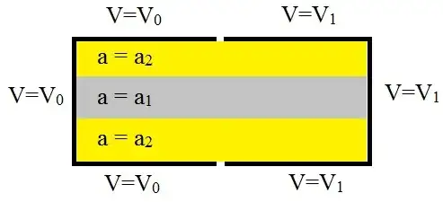
$\,A_y = \lambda/dy\cdot dx/2\,$ for the vertical edges, where $\lambda$ is the conductivity (equal to $a_1$ or $a_2$ in the OP's question). Resulting in the following "Finite Element matrix" for one rectangle: $$ \begin{bmatrix} A_x+A_y & - A_x & - A_y & 0 \\ - A_x & A_x+A_y & 0 & - A_y \\ - A_y & 0 & A_x+A_y & - A_x \\ 0 & - A_y & - A_x & A_x+A_y \end{bmatrix} $$ The rest of the numerical treatment is pretty standard Finite Element methodology:

program hesam;
Uses Laplace;
procedure test; var k : integer; begin Starten; {Initialize } for k := 0 to 9 do begin { FEM Calculations } Rekenen(Random,Random,0,1); { Store in 'results' file } Opschrijven(k); end; end;
begin test; end.
Here is a link to the complete (Delphi Pascal) unit that does the FEM Calculations:

Below is the $\,40\times 30\,$ grid that has been used for sample calculations and a contour map of some results with $V_0=0$ , $V_1=1$ and random $a_1,a_2$.

enter image description here

Sample output ('result' file) - can you see where it is? - :

   x   y       V[x,y]
  20   0  5.00000000000000E-0001
  20   1  5.00000000000000E-0001
  20   2  5.00000000000000E-0001
  20   3  4.99999999999999E-0001
  20   4  4.99999999999999E-0001
  20   5  4.99999999999999E-0001
  20   6  4.99999999999999E-0001
  20   7  4.99999999999999E-0001
  20   8  4.99999999999999E-0001
  20   9  5.00000000000000E-0001
  20  10  5.00000000000001E-0001
  20  11  5.00000000000001E-0001
  20  12  5.00000000000001E-0001
  20  13  5.00000000000002E-0001
  20  14  5.00000000000002E-0001
  20  15  5.00000000000002E-0001
  20  16  5.00000000000003E-0001
  20  17  5.00000000000003E-0001
  20  18  5.00000000000003E-0001
  20  19  5.00000000000002E-0001
  20  20  5.00000000000002E-0001
  20  21  5.00000000000003E-0001
  20  22  5.00000000000002E-0001
  20  23  5.00000000000002E-0001
  20  24  5.00000000000001E-0001
  20  25  5.00000000000001E-0001
  20  26  5.00000000000001E-0001
  20  27  5.00000000000001E-0001
  20  28  5.00000000000000E-0001
  20  29  5.00000000000000E-0001
  20  30  5.00000000000000E-0001
Han de Bruijn
  • 17,475
1

This is solvable with a Finite Fourier Transform in the $x$ coordinate. Without loss of generality, let $V_0=-1$ and $V_1=1$ (achievable with a simple shift and scale of the $V$ function). If we let $$ v_n(y) = \frac1b\int_{-b}^b V(x,y) \sin \left(\frac{n\pi x}{b}\right)dx $$ where we are neglecting the $\cos$ terms through the (anti-)symmetry of the system, then we have $$ V(x,y) = \sum_{n=1}^\infty v_n(y) \sin\left(\frac{n\pi x}b\right) $$ Now, we can see, through integration by parts, that $$ \frac1b\int_{-b}^b \frac{\partial^2 V}{\partial x^2}\sin\left(\frac{n\pi x}b\right)dx = -\frac{2n\pi(-1)^n}{b^2}-\frac{n^2\pi^2}{b^2}v_n(y) $$ Now, we're going to get rid of the $a$ variation by introducing boundaries. Assuming that the boundaries occur at $y_1$ and $y_2$, where $-c<y_1<y_2<c$, we will have the following boundary conditions at each of these boundaries: $$ V_1 = V_2 $$ and $$ a_1\mathbf{j}\cdot \nabla V_1 = a_2\mathbf{j}\cdot \nabla V_2 \qquad \text{or} \qquad a_1\frac{\partial V_1}{\partial y} = a_2\frac{\partial V_2}{\partial y} $$ which effectively says that the flux across the boundary from one side is equation to the flux across the boundary into the other side (if we interpret the equation as the steady state diffusion equation).

Now, as we can transform both of these equations in $x$ without changing their form, we can continue to apply these equations to the $v_n(y)$ functions. Applying our transform within each of the domains gives, $$ \frac{\partial^2 v_n}{\partial y^2}-\frac{n^2\pi^2}{b^2}v_n(y)=\frac{2n\pi(-1)^n}{b^2} $$ which has the general solution form $$ v_n(y) = \frac{2(-1)^{n+1}}{n\pi} + A_n\cosh\left(\frac{n\pi y}{b}\right)+B_n\sinh\left(\frac{n\pi y}{b}\right)\tag{1} $$ I'm not going to complete the process, but it's straightforward from here - transform the upper and lower boundaries so that they are boundaries in $v_n(y)$, then determine the $A_n$ and $B_n$ for each of the three domains by matching boundaries according to the above boundary condition setup. Note that the constant in (1) effectively produces $V_0(x,y) = \frac{x}b$, and is thus essentially accounting for the left and right boundaries.

Glen O
  • 12,743
  • Many thanks, Is it possible that the solution along x be in form of cosh(x) and sinh(x) and along y in form of sin(y)? I would like to see how the old solution would be recovered if we put $a_1$ = $a_2$ – Roy Feb 09 '15 at 18:48
  • 1
    It's somewhat harder to directly create it with that format, as we can't do an easy Fourier series transform on the $y$ coordinate of the problem. That being said, you can probably perform a Fourier series transform to the solution itself, although you'll probably have a double-summation and then have to show that, for $a_1=a_2$, the inner summation produces the functions seen in that old solution. Alternatively, you could repeat the old solution in reverse to get it in terms of $\sin(n\pi x/b)$. – Glen O Feb 10 '15 at 01:58
  • 1
    Note that it might be possible to create a generalised version of the transform, using Separation of Variables to determine the eigenfunctions, but there's no guarantee that they will be nice. – Glen O Feb 10 '15 at 02:00