Does exist a finite time when the probability of a Geometric Brownian Motion (GBM) crosses the path given by the median value becomes zero?

Question

Does exist a finite time when the probability of a Geometric Brownian Motion (GBM) crosses the path given by the median value becomes zero?

Intro

It is a well known fact that a Standard Brownian Motion (SBM) $W_t$ will visit the value zero infinitely often (check here - MSE). Here note that zero is the mean path $E[W_t]=0$ of the SBM.

Correct me if I am mistaken please, but my intuition tells me that this will mean that a Brownian Motion with Drift (DBM) $B_t = \mu t +\sigma W_t$ will cross the mean path given by $E[B_t] = E[\mu t]+E[\sigma W_t] = \mu t +\sigma \require{cancel}\cancel{E[W_t]}=\mu t$ infinitely often too, since is like a linear transformation of the SBM (kind of rotation of a SBM to the axis given by $E[B_t]=\mu t$).

But when thinking about the Geometric Brownian Motion (GBM) $X_t$ thinks get complicated, since the process is not ergodic anymore.

Motivation

If the GBM process is given by $X_t = X_0\exp\left(\left(\mu -\frac{\sigma^2}{2}\right)t +\sigma W_t\right)$ its probability distribution will be given by $P\left(X_t \leq x\right) = \Phi\left(\dfrac{\ln(x)-\ln(X_0)-\left(\mu -\frac{\sigma^2}{2}\right)t}{\sigma\sqrt{t}}\right)$ with $\Phi(\frac{x-a}{b})$ the standard normal cumulative distribution with mean value $a$ and standard deviation $b$.

Since the mean value path of the GBM is given by $E[X_t]= X_0 e^{\mu t}$ you could find that the long-term probability of been equal or higher the mean value path is zero: $$\begin{array}{r c l}P\left(X_t \geq X_0 e^{\mu t}\right) & = & 1 - P\left(X_t \leq X_0 e^{\mu t}\right) = 1 - \Phi\left(\dfrac{\cancel{\ln(X_0)}+\cancel{\mu t}-\cancel{\ln(X_0)}-\left(\cancel{\mu} -\frac{\sigma^2}{2}\right)t}{\sigma\sqrt{t}}\right) \\ & = & 1 -\Phi\left(\dfrac{\frac{\sigma^2}{2}t}{\sigma\sqrt{t}}\right) = 1 - \Phi\left(\frac{\sigma\sqrt{t}}{2}\right) \overset{t \to \infty}{=} 1 - 1 = 0\end{array}$$

Which tells me a few things: (i) I don't think would make too much sense to look for visiting the mean value path in the long term since there is zero probability to be over it as $t \to \infty$; and (ii) somehow in GBM the mean path value wouldn't be a representative path of the GBM path in the long term, since most of the paths would be below it.

In this sense, if instead I use as representative path of the GBM process the median value path $\theta_t = X_0\exp\left(\left(\mu -\frac{\sigma^2}{2}\right)t\right)$ at least I will know that for all times there is a $50/50$ chance of being over or below it.

At times near zero, all GBM paths would be near $X_0$ so is not nonsense to believe a path that started below $\theta_t$ could cross over it, and viceversa, but since as times grows the paths kind of become to be exponentially apart (at least those paths over the median value: think of the case of the mean value and median value paths, at $t \to \infty$, there $50\%$ of the sample paths would be among them), I believe that should there exist some finite time $T$ when, if I started below the median value I wouldn't be able to cross it again, and viceversa.

I hope the question makes sense. From the point of view of choosing stocks, if I estimate $\{\hat{X}_0,\ \hat{\mu},\ \hat{\sigma},\ \hat{T}\}$ and make an estimation of $\hat{\theta}_t$, it would be useful to know if at current time the value of the stock is below $\hat{\theta}_t$ and this current time is greater than $\hat{T}$, I will know beforehand that it would be highly improbable I will see this stock to grow as the estimated mean value path $e^{\hat{\mu}t}$.

---

---

Added later - not mandatory reading - Answering to @Snoop answer - too long for comment section

Reading the answer sees to me a completely valid way of reasoning, but somehow I don't fully understood I think that there is some assumption that is not valid from what simulations and other ways of seen the problem shows, which I would extend now.

While for a GBM variable $X_t$ the expected value is given by $E[X_t]=X_0e^{\mu t}$, the Median value is given by $\theta_t = X_0e^{\left(\mu -\frac{\sigma^2}{2}\right)t}$ (which split the trends in the $50/50$ probability), and the Mode Value will be given by $\nu_t = X_0e^{\left(\mu -\frac{3\sigma^2}{2}\right)t}$.

If I focus on the long term probability of being below the Mode value I will find:

$$\begin{array}{r c l}P\left(X_t \leq X_0 e^{\left(\mu-\frac{3\sigma^2}{2} \right)t}\right) & = & \Phi\left(\dfrac{\cancel{\ln(X_0)}+\cancel{\mu t}-\frac{3\sigma^2}{2}-\cancel{\ln(X_0)}-\left(\cancel{\mu} -\frac{\sigma^2}{2}\right)t}{\sigma\sqrt{t}}\right) \\ & = & \Phi\left(\dfrac{-\sigma^2t}{\sigma\sqrt{t}}\right) = \Phi\left(-|\sigma|\sqrt{t}\right) \overset{t \to \infty}{=} 0\end{array}$$

So from the Probability Distribution of a GBM I got that in the long term $50\%$ of the path will be between $E[X_t]$ and $\theta_t$, and the other $50\%$ of the path will be between $\theta_t$ and $\nu_t$, which makes very little sense for $\nu_t$ as Mode value unless it means that somehow $E[X_t]\to \theta_t$ and $\nu_t \to \theta_t$, which I now beforehand is not true. In this sense GBM is very weird, and somehow it tells the values are concentrated near the Median $\theta_t$ and not around the expected value $E[X_t]$.

This analysis, being weird, is somehow validating the answer deliver by @Snoop since is path are concentrated near the Median value at least there exist the possibility of crossing it if the path are wiggling around it.

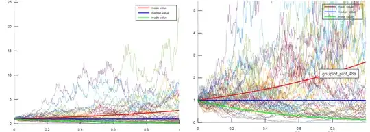
But unfortunately, is not hard to make a scenario to show GBM not always will follow these conclusions: let choose positive values $X_0 = 1$ such $\ln(X_0)=0$ just for cleaning it from the analysis, and $\{\mu,\ \sigma\}$ such they fulfill that $\mu-\frac{\sigma^2}{2}=0 \Rightarrow \mu:=\frac{\sigma^2}{2}$ so the median value $\theta_t = 1$ is constant, and also such as $\mu>1$ so the mean value $E[X_t]=e^{\mu t}$ is exponentially increasing (this implies $\frac{\sigma^2}{2}>1 \Rightarrow \sigma^2 > 2$), but such as $\mu-\frac32\sigma^2<0$ so the mode value $\nu_t = e^{\left(\mu -\frac32\sigma^2\right) t}$ is decreasing exponentially to zero (this is directly given since $\frac{\sigma^2}{2}-\frac{3\sigma^2}{2}= -\sigma^2 <0$). As you could check in Desmos this means the minimum values fulfilling these requirements are $(\mu,\ \sigma) = \left(1,\ \sqrt{2}\right)$. I simulate this scenario in Online Octave:

Here you could see how some path grows faster than the expected value while some decrease to zero somehow getting stuck at there (since every step will add very little at these level of the exponential).

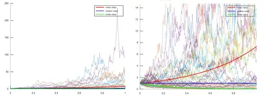
I can even make it worst as choosing $\mu-\frac12\sigma^2<0$ with $\mu >1$ so the expected value grows exponentially while the median an mode values $\{\theta_t,\ \nu_t\}$ decrease exponentially to zero as you could see in Desmos: in the following simulation I picked $(\mu,\ \sigma) = (2,\ 2)$, as you could see there are path over the mean value that hardly will decrease below it to match the decreasing Median value.

Somehow from the simulations it don't looks right neither obvious the paths would be crossing the Median Value infinitely often, maybe due the effect of the noise is dependent of how high is the previous value of the exponential trend maybe is not valid to think the process would fulfill analogous behaviors as of its argument (thinking on how the Inverse transform sampling works), but I don't really know, is like the GBM is following an exponential distribution instead of a log-normal distribution under these parameters.

Here I left the code I used:

#clear all; clc; clf;
length = 401; 
N = 50; 
dt=1/length;
white_noise = sqrt(dt)wgn(length-1,N,0); 
simple_brownian = zeros(length,N); 
t=0:1:length-1; 
t=dtt;
for m=1:1:N 
   simple_brownian(2:1:length,m) = cumsum(white_noise(:,m)); 
end
S0 = 1; 
sigma = sqrt(2); 
sigma2 = (sigma)^2; 
mu = 1/2*sigma2;
mean_val = S0exp(mut);

median_val = S0exp((mu-1/2sigma2)t); 
mode_val = S0exp((mu-3/2sigma2)t); 
GBM1 = ones(length,N);
for m=1:1:N 
   for k=1:1:length 
      GBM1(k,m) = S0exp((mu-1/2sigma2)t(k)+sigmasimple_brownian(k,m)); 
   end 
end
figure (1), 
hold on, 
plot(t,mean_val,'r','Linewidth',2,t,median_val,'b','Linewidth',2,t,mode_val,'g','Linewidth',2), legend('mean value','median value','mode value'), 
plot(t,GBM1), 
plot(t,mean_val,'r','Linewidth',2,t,median_val,'b','Linewidth',2,t,mode_val,'g','Linewidth',2), 
axis([0 t(length) 0 2S0exp(mu*(t(length)))]), 
hold off;
figure (2), 
hold on, 
plot(t,mean_val,'r','Linewidth',2,t,median_val,'b','Linewidth',2,t,mode_val,'g','Linewidth',2), legend('mean value','median value','mode value'), 
plot(t,GBM1), 
plot(t,mean_val,'r','Linewidth',2,t,median_val,'b','Linewidth',2,t,mode_val,'g','Linewidth',2), 
#axis([0 t(length) 0 2S0exp(mu*(t(length)))]), 
hold off; 

Answer 1

1D Brownian motion $W$ is point recurrent, so that it visits any given point infinitely many times for some sequence $t_n\uparrow \infty$, almost surely: formally, if we choose zero then $P(\exists (t_n)_n:t_n\uparrow \infty,W_{t_n}=0)=1$. So, for example, if $X_t:=\mu t+\sigma W_t$ then $\frac{X_t-\mu t}{\sigma}=W_t$ visits zero infinitely many times for some sequence $t_n\uparrow \infty$, so $P(\exists (t_n)_n:t_n\uparrow \infty,X_{t_n}=\mu {t_n})=1$. If we consider the GBM $Y_t=y_0\exp((\mu-\sigma^2/2)t+\sigma W_t),y_0>0$ then we can also notice that $\frac{\ln(Y_t/y_0)-(\mu-\sigma^2/2)t}{\sigma}=W_t$ so we have that $P(\exists (t_n)_n:t_n\uparrow \infty,Y_{t_n}=y_0 e^{(\mu-\sigma^2/2)t_n})=1$ so $Y$ crosses the 'median path' $(y_0e^{(\mu-\sigma^2/2)t})_{t\geq 0}$ infinitely many times for some sequence $t_n\uparrow \infty$, almost surely.