Simulating a Function (that is naturally contained) Within an Interval $a,b$

Question

I am trying to learn how to mathematically define and simulate a Stochastic Process such that it "naturally" only remains between two points $(a,b)$.

Based on a previous question I posted (How to Contain a Brownian Motion Between 2 Points?), it was suggested to me in this answer (https://math.stackexchange.com/a/4828166/791334) that I should consider modifying the Ornstein-Uhlenbeck process (https://en.wikipedia.org/wiki/Ornstein%E2%80%93Uhlenbeck_process - note that the Ornstein-Uhlenbeck process is based on the Weiner Process).

Here is my attempt to unpack this information and simulate a Stochastic Process between two points $(a,b)$. First, I will try to mathematically define the Wiener Process, the Ornstein-Uhlenbeck process and the modified Ornstein-Uhlenbeck Process between the interval $(a,b)$ in Part 1 - then, I will try to perform the corresponding simulations for these processes (using the R programming language) in Part 2.

Part 1: Definitions

1. Wiener Process: As I understand, the Wiener Process $W_t$ can be thought of as successive differences between a Brownian Motion. Here are some standard properties about to Brownian Motion:

   • $W_0 = 0$ almost surely.
   • $W$ has independent increments: for every $t > 0$, the future increments $W_{t+u} - W_t$, $u \geq 0$, are independent of the past values $W_s$, $s < t$.
   • $W$ has Gaussian increments: $W_{t+u} - W_t$ is normally distributed with mean 0 and variance $u$, $W_{t+u} - W_t \sim N(0, u)$.

2. Ornstein-Uhlenbeck Process: The Ornstein-Uhlenbeck process $X_t$ is defined by the following stochastic differential equation:

$$dx_t = \theta (\mu - x_t) \, dt + \sigma \, dW_t$$

where:

• $\theta > 0$ and $\sigma > 0$ are parameters
• $W_t$ denotes the Wiener process.
• $\mu$ is a drift constant.

If I understand correctly, the Ornstein-Uhlenbeck process can be "discretized" (via the Euler-Maruyama method) as follows:

$$X_{t+\Delta t} = X_t + \theta (\mu - X_t) \Delta t + \sigma \Delta W_t$$

Note: My "naive" way of understanding the original Ornstein-Uhlenbeck process $dx_t = \theta (\mu - x_t) \, dt + \sigma \, dW_t$ is that (for constant small, time intervals), $dt = 0.01$, $dW_t$ is the difference in the Wiener Process between some small interval $dt = 0.01$. Thus, approximately, $dx_t = \theta (\mu - x_t) \, *0.01 + \sigma \, dW_t$

3. Modifying the Ornstein-Uhlenbeck process to be constrained between two points $(a,b)$:

In this answer (https://math.stackexchange.com/a/4828166/791334), I learned that the Ornstein-Uhlenbeck process can transformed into a new process $Y_t$ that will now be contained between $(0,1)$:

$Y_t = \frac{e^{X_t}}{1 + e^{X_t}}$

By scaling $Y_t$, I think we should now be able to define it between two points $(a,b)$:

$$Y_t = a + \left(\frac{e^{X_t}}{1 + e^{X_t}}\right) \cdot (b - a)$$

Thus, we can outline a simulation algorithm based on theory:

• Calculate time increment $\Delta t = t[i] - t[i-1]$.
• Simulate the Wiener process increment $\Delta W \sim N(0, \sqrt{\Delta t})$.
• Calculate the Ornstein-Uhlenbeck process increment:

$$\Delta X = \theta (\mu - X[i-1]) \Delta t + \sigma \Delta W$$

• Update the Ornstein-Uhlenbeck process:

$$X[i] = X[i-1] + \Delta X$$

• Transform the Ornstein-Uhlenbeck process to get the process $Y$ that is constrained between $(a, b)$:

$$Y[i] = a + \left(\frac{e^{X[i]}}{1 + e^{X[i]}}\right) \cdot (b - a)$$

• Note, if we want the transformed process to start at a specific point $Y_0 = y_0$, we can write the corresponding $x_0$ such that:

$$y_0 = a + \left(\frac{e^{x_0}}{1 + e^{x_0}}\right) \cdot (b - a)$$

$$x_0 = \ln\left(\frac{y_0 - a}{b - y_0}\right)$$

Part 2: Simulations

Now, I will try to simulate these processes using the R programming language.

1. Simulating the Wiener Process:

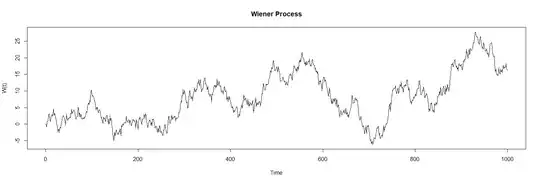
We can that even though this process is centered around a Normal Distributions of mean=0, it still exceeds the range $(0,1)$:

t <- seq(0, 1000, by = 1)  # Time points
Initialize
W <- numeric(length(t))
W[1] <- 0
Simulate
set.seed(123)

for (i in 2:length(t)) {
    dt <- t[i] - t[i-1]
    dW <- rnorm(1, mean = 0, sd = sqrt(dt))

    W[i] <- W[i-1] + dW
}
plot(t, W, type = "l", main = "Wiener Process", xlab = "Time", ylab = "W(t)")

2. Simulating the Ornstein-Uhlenbeck Process:

theta <- 1  # Mean reversion constant
mu <- 0     # Long-term mean
sigma <- 1  # Volatility
x0 <- 0     # Initial position
t <- seq(0, 1000, by = 1)  # Time points
Initialize
X <- numeric(length(t))
X[1] <- x0
Simulate the process
set.seed(123) 
for (i in 2:length(t)) {
    dt <- t[i] - t[i-1]
    dW <- rnorm(1, mean = 0, sd = sqrt(dt))  # Wiener process
    dX <- theta * (mu - X[i-1]) * dt + sigma * dW
    X[i] <- X[i-1] + dX
}
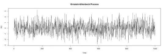
plot(t, X, type = "l", main = "Ornstein-Uhlenbeck Process", xlab = "Time", ylab = "X(t)")

3. Simulating a Process that never exceeds (a,b):

Based on the above simulation, here is a process that should never exceed $a = 6$ and $b=8.3$

t <- seq(0, 10000, by = 1)
theta <- 1  # Mean reversion constant
mu <- 0     # Long-term mean
sigma <- 1  # Volatility
a <- 6      # Lower bound
b <- 8.3    # Upper bound
y0 <- 7     # Desired starting point for Y
initial condition for X
x0 <- log((y0 - a) / (b - y0))
Initialize
X <- numeric(length(t))
X[1] <- x0
Y <- numeric(length(t))
Y[1] <- y0
Simulate
set.seed(123) 
for (i in 2:length(t)) {
    dt <- t[i] - t[i-1]
    dW <- rnorm(1, mean = 0, sd = sqrt(dt))  # Wiener process
    dX <- theta * (mu - X[i-1]) * dt + sigma * dW
    X[i] <- X[i-1] + dX
    Y[i] <- a + (exp(X[i]) / (1 + exp(X[i]))) * (b - a)  # Transformation
}
plot(t, Y, type = "l", main = "Transformed Ornstein-Uhlenbeck Process", xlab = "Time", ylab = "Y(t)")

Empirically, we can see that based on a large number of iterations, the process never exceeds the ranges we specified. Thus, this transformed process only remains "naturally" between points $a,b$.

My Question: Have I done this correctly?

Thanks!

Answer 1

Glad you got your simulation working. Yes this is exactly what I was suggesting in the previous answer.

It's interesting to see that you have scaled and recentered the modified process $Y$, given that you mentioned modeling a probability originally. My original intention with the transform $e^{X_t}/(1 + e^{X_t})$ was so that $X_t$ would have a natural interpretation as log-odds.

If you don't need this property, there are much simpler transforms you can do. You could directly transform the Weiner process. Take $Y_t = \sin^2(W_t)$ for example, or $Y_t = T(W_t)$ where $T$ is the triangle wave.

You could take a look at what kinds of sample paths these give you to see if they suit your application.