How to Contain a Brownian Motion Between 2 Points?

Question

I am interested in learning about if it is possible to mathematically define a Brownian Motion such that it can ONLY take values between two points $a$ and $b$.

Part 1: Definition

Consider a Wiener Process (https://en.wikipedia.org/wiki/Wiener_process):

A Wiener process $W(t)$, $t \in [0, \infty)$, is a real-valued continuous-time stochastic process that satisfies the following properties:

1. $W_0 = 0$
2. $W$ has independent increments: for every $t > 0$, the future increments $W_{t+u} - W_t$, $u \geq 0$, are independent of the past values $W_s$, $s < t$.
3. $W$ has Gaussian increments: $W_{t+u} - W_t$ is normally distributed with mean 0 and variance $u$, i.e., $W_{t+u} - W_t \sim \mathcal{N}(0, u)$.

Thus, in general:

$$W(t) = \sum_{i=1}^{t-1} (W_i - W_{i-1})$$ $$(W_i - W_{i-1}) \sim \mathcal{N}(0, dt)$$

Part 2: Simulating a Basic Process

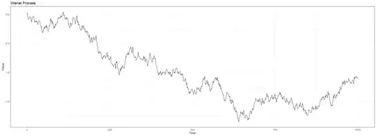
Here is my attempt to simulate a Wiener Process in the R programming language:

library(ggplot2)
n <- 1000  # Number of steps
dt <- 1/n  # Time step
dW <- rnorm(n, mean = 0, sd = sqrt(dt))
W <- cumsum(dW)
df <- data.frame(time = seq(0, 1000, length.out = n), Wiener = W)
p <- ggplot(df, aes(x = time, y = Wiener)) +
    geom_line() +
    labs(title = "Wiener Process", x = "Time", y = "Value") + theme_bw()
print(p)

Part 3: Manually Forcing a Brownian Motion to stay between two points:

For example, imagine a coin where the probability of success itself evolves as a stochastic process. That is, the probability of getting heads on the $n_{th}$ turn depends on the history of the previous flips according to a Wiener Process. In this case, I would have to define a Wiener Process between $0$ and $1$.

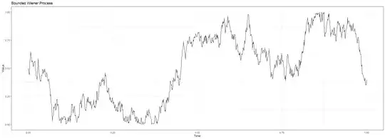
From a programming perspective, I think this might be possible: Every time the Wiener Process takes a value of $0$ or $1$, you can "force" it to take a value of 0.01 or 0.99 and resume the simulation:

n <- 1000  # Number of steps
dt <- 1/n  # Time step
dW <- rnorm(n, mean = 0, sd = sqrt(dt))
W <- numeric(n)
W[1] <- 0.5  # Start in the middle of the interval [0, 1]
Generate the Wiener process
for (i in 2:n) {
  W[i] <- W[i-1] + dW[i]
If the process hits 0 or 1, reset to 0.01 or 0.99 respectively
if (W[i] <= 0) {
    W[i] <- 0.01
  } else if (W[i] >= 1) {
    W[i] <- 0.99
  }
}
df <- data.frame(time = seq(0, 1, length.out = n), Wiener = W)
p <- ggplot(df, aes(x = time, y = Wiener)) +
  geom_line() +
  labs(title = "Bounded Wiener Process", x = "Time", y = "Value") +
  theme_bw()
print(p)

Part 4: Reflected Brownian Motion

I found this link (https://en.wikipedia.org/wiki/Reflected_Brownian_motion) which looks that it might be possible to "bound" a Brownian Motion (quoting the Wikipedia Page):

A $d$-dimensional reflected Brownian motion $Z$ is a stochastic process on $\mathbb{R}^d_+$ uniquely defined by:

• a $d$-dimensional drift vector $\mu$,
• a $d \times d$ non-singular covariance matrix $\Sigma$
• a $d \times d$ reflection matrix $R$.

Where:

• $X(t)$ is an unconstrained Brownian motion with drift $\mu$ and variance $\Sigma$
• $Z(t) = X(t) + R Y(t)$

Such that: $Y(t)$ a $d$-dimensional vector where:

• $Y$ is continuous and non-decreasing with $Y(0) = 0$,
• $Y_j$ only increases at times for which $Z_j = 0$ for $j = 1,2,...,d$,
• $Z(t) \in \mathbb{R}^d_+$, $t \geq 0$.

But, from the above text, it seems like $Z(t) = X(t) + R Y(t)$ is the general form for a "constrained" (i.e. reflected) Brownian Motion - however, within this formulation, I am not sure which boundaries (i.e. values of a,b) this Brownian Motion will be contained within. Furthermore, I am not sure how the matrix $R$ needs to be defined such that the Brownian Motion lies between $(a,b)$.

My Question: How can I mathematically define the Wiener Process such that the range can only be between two numbers $a$ and $b$?

Thanks!

Note: Just to clarify - I want to ensure that the Brownian Motion NEVER exceeds a value of $a,b$ ... I am not interested in the concept of the "Brownian Bridge"(https://en.wikipedia.org/wiki/Brownian_bridge) where the Brownian Motion takes a value of 0 at time=0 and time=T.

Answer 1

The most natural way to force the Wiener process $W$ to stay in the interval $[0,1]$ is via conditioning. In other words, you consider a new process $\hat{W}$ which is $W$ conditioned on $W_t \in [0,1]$ for all $t$. (This can be rigorously done using Doob's h-transform). This process is solution to the SDE $$d\hat{W}_t = dW_t + \pi \cot(\pi \hat{W}_t)dt.$$ Notice the drift is $+\infty$ when $\hat{W}_t = 0$ forcing the process to increase and similarly when $\hat{W}_t = 1$.

To simulate it, either discretize the SDE or even simpler: knowing the value $\hat{W}_{t_i}$, to get $\hat{W}_{t_{i+1}}$, keep generating random variables $Z$ with distribution $N(0,t_{i+1}-t_i)$ until $\hat{W}_{t_i} + Z \in [0,1]$; this will be $\hat{W}_{t_{i+1}}$.

Answer 2

You might consider taking $Y_t = \frac{e^{X_t}}{1 + e^{X_t}}$ where $X_t$ is an Ornstein Uhlenbeck process. Then $X_t$ would have natural interpretation as a log odds prior whose long term limit is normally distributed at zero, and $Y_t \in [0,1]$ would have natural interpretation as a probability.

Through the Ito Lemma, you could recover the SDE for $Y_t$ in terms of the Weiner process, if you needed.