$\int_0^\infty \frac{u^5 \, J_0\left( u\right)}{\left( u^2+x^2 \right)^{1/2}}\,e^{- u-\left( u^2+x^2 \right)^{1/2} }\,\mathrm{d}u $

Question

Consider the following infinite integral that emerged while solving a fluid physical problem involving viscous flow in porous media: $$ f(x) = \int_0^\infty \frac{u^5 \, J_0 \left( u\right) }{\left( u^2+x^2 \right)^{1/2}} \, e^{- u-\left( u^2\,+\,x^2 \right)^{1/2}} \, \mathrm{d} u \, , $$ wherein $x \in \mathbb{R}$ is the real variable. Here, $J_0$ denotes the zeroth-order Bessel function of the first kind.

While a closed analytical expression might most likely be delicate and far from being trivial, I was wondering whether the above integral can potentially be transformed into a single infinite sum.

What I tried is to use the following infinite series expansion of the Bessel function: $$ J_0 (u) = \sum_{m \ge 0} \frac{(-1)^m}{m!^2} \left( \frac{u}{2} \right)^{2m} \, , $$ together with $$ e^{-\left( u^2\,+\,x^2 \right)^{1/2}} = \sum_{n \ge 0} \frac{(-1)^n}{n!} \left( u^2+x^2 \right)^{n/2} \, , $$ leading to a double sum, which does not seem to be converging to the original function for some reason.

Alternatively, I tried to use Poisson's integral to write the Bessel function in the form $$ J_0(u) = \frac{2}{\pi} \int_0^1 \frac{\cos uv}{\left(1-v^2\right)^{1/2}} \, \mathrm{d} v $$ and interchange the order of integration. Unfortunately this trick also does not seem to be of great help.

Any hints would be highly appreciated. Thank you!

In particular, for $x=0$, it can readily be shown that $$ f(0) = \frac{21 \sqrt{5}}{625} \, . $$

Answer 1

Consider the integral $$ I(x,s) = \int_0^\infty \!\!\! u^5 \, J_0 \left( u\right) \, \mathrm{e}^{- su}\dfrac{\mathrm{e}^{-\sqrt{u^2+x^2}}}{\sqrt{u^2+x^2}} \, \mathrm{d} u ,\quad \text{with}\quad x \in \mathbb{R}, $$ in which we have inserted a parameter $s$ to represent a Laplace transform. The integral required is then $I(x,1).$

If we denote by $I_{1}(x,s)$ the integral which contains $u$ instead of $u^5,$ the integral could also be found by taking ${\rm d}^4 I_{1}(0,s)/{\rm d}s^4$ and setting $s=1$ in the resulting transform. We then recover the OP's result, $I(0,1)=\left[{\rm d}^4 I_{1}(0,s)/{\rm d}s^4\right]_{s=1}=21\sqrt{5}/625.$

We now consider the original integral without the $s$ parameter, $$ \int_0^\infty \!\!\! u^5 \, J_0 \left( u\right) \, \mathrm{e}^{- u}\dfrac{\mathrm{e}^{-\sqrt{u^2+x^2}}}{\sqrt{u^2+x^2}} \, \mathrm{d} u ,\quad \text{with}\quad x \in \mathbb{R}, $$ and attempt to morph it into a form suitable for table lookup, or computer algebra evaluation.

Put $$ \varpi=u+\sqrt{u^2+x^2}\tag{1}.$$ On differentiation $$\dfrac{{\rm d}\varpi}{{\rm d}u} =1+\dfrac{u}{\sqrt{u^2+x^2}}=\dfrac{u+\sqrt{u^2+x^2}}{\sqrt{u^2+x^2}}= \dfrac{\varpi}{\sqrt{u^2+x^2}},\, $$ or $$ \dfrac{{\rm d}\varpi}{\varpi} = \dfrac{{\rm d }u}{\sqrt{u^2+x^2}}\tag{2} .$$ On inversion, $(1)$ gives $$u=\dfrac{\varpi^2-x^2}{2\varpi}\tag{3}. $$ Inserting these results into the integral and changing the limits, gives $$I(x)=\int_{x}^{\infty}\left(\dfrac{\varpi^2-x^2}{2\varpi}\right)^{\!5} J_0\!\left(\dfrac{\varpi^2-x^2}{2\varpi}\right)\!\dfrac{{\rm e}^{-\varpi}}{\varpi}\,{\rm d}\varpi.$$

We now reintroduce the $s$ parameter and consider the Laplace transform integral $$I(x,s)=\int_{x}^{\infty}\left(\dfrac{\varpi^2-x^2}{2\varpi}\right)^{\!5} J_0\!\left(\dfrac{\varpi^2-x^2}{2\varpi}\right)\!\dfrac{{\rm e}^{-s\varpi}}{\varpi}\,{\rm d}\varpi\tag{4},$$ where we will eventually set $s=1.$

The Bessel function $J_{0}(z-\varepsilon)=J_{0}(z)-\varepsilon J_{0}^{'}(z)+\varepsilon^2 J_{0}^{''}(z)/2!+\mathcal{O}(\varepsilon^3)$ can be expanded in a Taylor series about the point $z=\varpi/2$, with primes denoting differentiation with respect to $z$, and putting $z=\varpi/2$ and $\varepsilon=x^2/(2\varpi),$ we get $$ J_0\!\left(\dfrac{\varpi^2-x^2}{2\varpi}\right)=J_0\!\left(\dfrac{\varpi}{2}\right) - \left(\!\dfrac{x^2}{2\varpi}\!\right)\!J_1\!\left(\dfrac{\varpi}{2}\right)- \left(\!\dfrac{x^2}{2\varpi}\!\right)^{\!\!2}\! \left( \!\dfrac{J_{0}\left(\varpi/2\right)-J_{2}\left(\varpi/2\right)}{4} \right)+\mathcal{O}\left(\!\! \left( \dfrac{x^2}{2\varpi}\! \right)^{\!\!3} \, \right), $$ where the recursion and differential relations for the Bessel function $J_{0}(x)$ have been used.

The term raised to the 5th power, on dividing by the $\varpi$ under the exponential, can be written as $$ \dfrac{1}{\varpi}\left(\dfrac{\varpi^2-x^2}{2\varpi}\right)^{\!5} =\left( \dfrac{\varpi^4}{2^5}\right)\!\left(1-5\left(\!\dfrac{x}{\varpi}\!\right)^{\!2} +10 \left(\!\dfrac{x}{\varpi}\!\right)^{\!4} -10\left(\!\dfrac{x}{\varpi}\!\right)^{\!6} +5 \left(\!\dfrac{x}{\varpi}\!\right)^{\!8} - \left(\!\dfrac{x}{\varpi}\!\right)^{\!10}\,\,\right). $$

The idea then is to pick out the terms in $$\dfrac{1}{\varpi}\left(\dfrac{\varpi^2-x^2}{2\varpi}\right)^{\!5} J_0\!\left(\dfrac{\varpi^2-x^2}{2\varpi}\right)\tag{5},$$ for which $\varpi^m$ has $m\ge 0.$ If $m<0$ the Laplace transforms with these terms will diverge, as noted by the OP, although the transforms with large order $n$ in $J_{n}(\varpi/2)$ in the Taylor series of the Bessel function do allow negative powers of $\varpi,$ up to a certain order. For example, the Laplace transforms of $J_{n}(\varpi/2)/\varpi^n$ can be computed. We ignore this and simply split the integrand in $(5)$ up into those terms with $m\ge 0$ and those for which $m<0$.

If we denote the terms with $\varpi^m$ satisfying $m\ge 0$ as $S_{\,p}$, and those for which $m<0$ as $S_{\,n}$, then $$\dfrac{1}{\varpi}\left(\dfrac{\varpi^2-x^2}{2\varpi}\right)^{\!5} J_0\!\left(\dfrac{\varpi^2-x^2}{2\varpi}\right)=S_{\,p}+S_{\,n}\tag{6}.$$ We can take the Laplace transforms of the terms in $S_{\,p},$ but not of those in $S_{\,n}.$ The terms in $S_{\,n}$ can be expanded entirely in powers of $\varpi^{m}$ and we will have integrals (with $s=1$) of the form $$\int_{x}^{\infty} \varpi^{m}\, {\rm e}^{-\varpi}\,{\rm d}\varpi=\Gamma(m+1,x)\tag{7}, $$ from Grashteyn & Rhyzik, page $940, 8.350, \#2.$

The integrals in $S_{\,p}$ involving integration from $\varpi=x$ to $\varpi=\infty$ can be split into an integral from $0$ to $\infty$ minus an integral from $0$ to $x,$ and will have the form $$\begin{align*}& \int_{x}^{\infty} \varpi^m J_{n}(\varpi/2)\,{\rm e}^{-s\varpi}\,{\rm d}\varpi=\! \int_{0}^{\infty} \varpi^m J_{n}(\varpi/2)\,{\rm e}^{-s\varpi}\,{\rm d}\varpi -\!\int_{0}^{x} \varpi^m J_{n}(\varpi/2)\,{\rm e}^{-s\varpi}\,{\rm d}\varpi \\ &=\dfrac{\Gamma(n+m+1)}{\left(s^2+1/4\right)^{\frac{m+1}{2}}}P_{\,\,\,m}^{-n}\left(\dfrac{s}{\sqrt{s^2+1/4}}\right)-\!\int_{0}^{x} \varpi^m J_{n}(\varpi/2)\,{\rm e}^{-s\varpi}\,{\rm d}\varpi\tag{8},\\ \end{align*} $$ where $P_{\,\,\,m}^{-n}\left(\dfrac{s}{\sqrt{s^2+1/4}}\right)$ is an associated Legendre function, Gradshteyn & Rhyzik, page $711, \#6.621, {\rm ET}\,{\rm II}\ 29(6).$ The Bessel function in the last integral from $0$ to $x$ can be expanded in powers of $\varpi$ and integrated term by term in a series with the help of $(7)$. In (8) we must put $s=1.$

We can now consider the integration of the series $S_{\,p}.$ From $(5),$ the first few terms up to $x^2,$ with positive $\varpi$ powers in $S_{\,p},$ are $$\dfrac{\varpi^4}{2^5}\left(J_{0}\left(\dfrac{\varpi}{2}\right) -\dfrac{5x^2}{\varpi^2}J_{0}\left(\dfrac{\varpi}{2}\right)-\dfrac{x^2}{2\varpi}J_{1}\left(\dfrac{\varpi}{2}\right) \right), $$ and putting this into the integral from $\varpi=0$ to $\varpi=\infty$ gives $$I(x,s)\approx\int_{0}^{\infty}\dfrac{\varpi^4}{2^5}\left(J_{0}\left(\dfrac{\varpi}{2}\right) -\dfrac{5x^2}{\varpi^2}J_{0}\left(\dfrac{\varpi}{2}\right)-\dfrac{x^2}{2\varpi}J_{1}\left(\dfrac{\varpi}{2}\right) \right) \!{\rm e}^{-s\varpi}\,{\rm d}\varpi\tag{9}.$$ On performing these Laplace transforms with wxmaxima, it avoids the associated Legendre polynomials and gives directly $$I(x,s)\approx $$ $$ {{{{24\,\left(-{{5}\over{4\,\left({{1}\over{4\,s^2}}+1\right)^{{{7 }\over{2}}}\,s^2}}+{{35}\over{128\,\left({{1}\over{4\,s^2}}+1\right) ^{{{9}\over{2}}}\,s^4}}+{{1}\over{\left({{1}\over{4\,s^2}}+1\right) ^{{{5}\over{2}}}}}\right)}\over{s^5}}-{{10\,\left({{1}\over{\left({{ 1}\over{4\,s^2}}+1\right)^{{{3}\over{2}}}}}-{{3}\over{8\,\left({{1 }\over{4\,s^2}}+1\right)^{{{5}\over{2}}}\,s^2}}\right)\,x^2}\over{s^ 3}}}\over{32}}+\left(1-\sqrt{{{1}\over{4\,s^2}}+1}\right)\,s\,x^2, $$ and on putting $s=1$ in this result we obtain

$$I(x,1)\approx {{21}\over{5^{{{7/2}}}}}+\dfrac{(4\times 5^{3/2}-57)x^2}{(4\times 5^{3/2})}.$$ Note that this is just the Laplace transform of the first few terms in $S_{\,p},$ and does not include contributions from the other integral over the limits $0$ to $x$ in $S_{\,p},$ or from the terms in $S_{\,n}.$

This is a quick preliminary result, pointing out the way I proceeded and can hardly be called a canonical series solution. I have not checked the results and will attempt a more in depth treatment when I have time. Would contour integration produce a neater result?

Edit

The required integral is $$ I(x) = \int_0^\infty \!\!\! u^5 \, J_0 \left( u\right) \, \mathrm{e}^{-u}\dfrac{\mathrm{e}^{-\sqrt{u^2+x^2}}}{\sqrt{u^2+x^2}} \, \mathrm{d} u ,\quad \text{with}\quad x \in \mathbb{R}. $$ The preceding answer is only valid for small values of $x, $ because the Taylor expansion was made about the point $\varpi/2.$ The OP requested that the expansion should hold for arbitrary values of $x$, and a series expansion valid for arbitrary $x$ is given below.

A plot of the integrand's variation with $u$ for several values of $x$ is shown in the following figure,

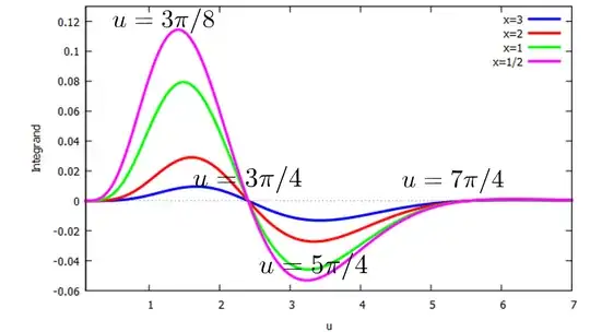
where it can be seen that it crosses the $u$-axis at the zeros of the Bessel function $J_{0}(u).$ For $u>1,$ the Bessel function is well represented by the asymptotic expansion $$J_{0}(u)\approx \sqrt{2/(\pi x)}\cos(u-\pi/4),$$ which crosses the $u$-axis at the zeros of the cosine function at $$u=3\pi/4, 7\pi/4, 11\pi/4, 15\pi/4, 19\pi/4, 23\pi/4\dots,$$ or at $$u_{n}=\left(n-\tfrac{1}{4}\right)\pi,\quad n=1,2,3,\ \dots.$$ From the figure we see that the integrand rises to maximum and minimum values approximately half-way between these zeros, approximately at the points $$ u_{n}^{\rm max,min} =3\pi/8, 5\pi/4, 9\pi/4, 13\pi/4, 17\pi/4, 21\pi/4,\dots.$$ or, after the first maximum, by $$u^{\rm max,min }_{n}= \left(n+\tfrac{1}{4}\right)\pi ,\quad n=1,2,3,\ \dots$$ Since the integrand is expanded in each region and then integrated over the regions between each zero of the cosine function, no error is committed in the integration by taking approximate zeros and approximate maxima/minima, and then expanding the integrand in a Taylor series about each of the maxima/minima.

Denote the integrand as $$ f(u,x)\,{\rm e}^{-u}\quad \text{ where }\quad f(u,x)=u^5 J_{0}(u)\,\dfrac{{\rm e}^{-\sqrt{u^2+x^2\vphantom{L^Y}}}}{\sqrt{u^2+x^2\vphantom{L^Y}}}.$$ In the integral from $\left(n-\frac{1}{4}\right)\!\pi$ to $\left(n+\frac{3}{4}\right)\!\pi,$ the integrand can be approximated by a Taylor series expansion in powers of $\Bigl(u-\left(n+\tfrac{1}{4}\right) \Bigr)^{\!m}$ about $u^{\rm max,min }_{n}=\left(n+\tfrac{1}{4}\right)\pi,\vphantom{\int\limits^{Y} }$ and the integral of $ f(u,x)\,{\rm e}^{-u}$ can then be written as $$ I(x)= \sum_{m=0}^{\infty}\,\int_{0}^{\frac{3}{4}\pi}\, \dfrac{1}{m!} \left[\dfrac{{\rm d}^m f(u,x)}{{\rm d}u^m}\right]_{u=\tfrac{3\pi}{8}}\Bigl(u-\tfrac{3\pi}{8}\Bigr)^{\!m}{\rm e}^{-u}\,{\rm d}u$$ $$ + \sum_{n=1}^{\infty}\sum_{m=0}^{\infty}\,\int_{\left(n-\frac{1}{4}\right)\pi}^{\left(n+\frac{3}{4}\right)\pi}\,\dfrac{1}{m!} \left[\dfrac{{\rm d}^m f(u,x)}{{\rm d}u^m}\right]_{u= \left(n+\tfrac{1}{4}\right)\pi }\Bigl(u-\left(n+\tfrac{1}{4}\right)\pi \Bigr)^{\!m}{\rm e}^{-u}\,{\rm d}u, $$ or as $$ I(x)= \sum_{\!n=0}^{\!\infty} \sum_{m=0}^{\infty}\,\int_{\theta(n)}^{\theta(n+1)}\,\dfrac{1}{m!} \left[\dfrac{{\rm d}^m f(u,x)}{{\rm d}u^m}\right]_{u= \phi(n) }\Bigl(u-\phi(n) \Bigr)^{\!m}{\rm e}^{-u}\,{\rm d}u, $$ where $$ \theta(n)=\begin{cases} 0 &\text{for}\,\, n=0, \\ \left( n-\tfrac{1}{4} \right)\pi& \text{for}\,\,n>0, \end{cases} $$ and $$ \phi(n)=\begin{cases} 3\pi/8 &\text{for}\,\, n=0, \\ \left( n+\tfrac{1}{4} \right)\pi& \text{for}\,\,n>0. \end{cases} $$ Because the $m$th order derivative terms in the square braces are independent of the integration variable $u,$ we have to evaluate simple integrals of the form $$E(n,m)=\int_{\left(n-\frac{1}{4}\right)\pi}^{\left(n+\frac{3}{4}\right)\pi}\,\Bigl( u-\left(n+\tfrac{1}{4}\right)\pi \Bigr)^{\!m}\,{\rm e}^{-u}\,{\rm d}u = {\rm e}^{-\left(n+\frac{1}{4}\right)\pi}\left[ \Gamma\left(m+1,-\frac{\pi}{2}\right)-\Gamma\left(m+1,\frac{\pi}{2}\right) \right] ,\quad n=1,2,3,\dots$$ where $\Gamma(m,z)$ is the incomplete gamma function. The case when $n=0$ is given by $$E(0,m)= \int_{0}^{\frac{3\pi}{4}}\,\left( u-\tfrac{3\pi}{8} \right)^{m}\,{\rm e}^{-u}\,{\rm d}u ={\rm e}^{-3\pi/8}\left[\Gamma(m+1,0)-\Gamma(m+1,3\pi/4)\right] ,$$ so that $$ I(x)= \sum_{\!n=0}^{\!\infty} \sum_{m=0}^{\infty}\,\dfrac{E(n,m)}{m!} \left[\dfrac{{\rm d}^m f(u,x)}{{\rm d}u^m}\right]_{u=\phi(n) }. $$

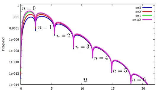
To evaluate the series, we truncate the evaluations at $n=6$ and $m=12.$ The reason can be seen in the following figure, which shows that the contribution of the integrand is negligible beyond $n=6.$ It was found that the Taylor series expansions of the integrand between the zeros of the cosine function need to be evaluated to $12$ terms in order for a plot of the exact and Taylor series representation of the integrand to overlap. This produces the results below, where the "Exact Integral" was evaluated using numerical integration. Taking more terms in the summations will increase the accuracy of the values in the following table:

$$ \begin{array}{c|cc} x & {\rm Exact\ Integral} & {\rm Approximate\ Integral\ Taylor\ Series} \\ \hline 0 &+ 0.07513188 & + 0.07513837 \\ 1/2 &+ 0.05305242 & + 0.05297258 \\ 1 &+ 0.01941515 & + 0.01912568 \\ 2 & - 0.01081567 & - 0.01072560 \\ 3 & -0.01060124 & - 0.01059756 \\ 4 &- 0.00571464 & - 0.00571490 \\ 5 & - 0.00253282 & - 0.00253294 \\ 10 & - 1.89475801 \times 10^{-5} & - 1.89482719\times 10^{-5} \\ 50 &-2.26246490 \times10^{-23} & - 2.26248108\times10^{-23} \\ 100 &-2.15544245 \times10^{-45} &- 2.15562626\times 10^{-45 } \\ \end{array}$$

The plots and integral evaluation in wxmaxima are given below:

The zeros of the integrand occur at the zeros of $J_{0}(u),$ at $u=2.4, u=5.5,$ etc. After the first four zeros, the integrand is approximately zero, so only the maxima shown in the following plots contribute to the integral. The maxima occur at the zeros of $J_{0}'(u)=0,$ at $u_{0}, u_{1},$ etc. Since the Bessel function $J_{0}(u)$ is approximately a decaying cosine when $u>1,$ we may approximate the zeros of $J_{0}(u)$ with the roots of $\cos(u-\pi/4),$ and these are used below. The maximums are taken midway between the approximate zeros of $\cos(u-\pi/4).$ Since the integrand is expanded in each region and then integrated over the regions between each root, no error is committed in the integration by taking approximate roots and maxima, since Taylor expansions can be taken about any point that is convenient and well represents the integrand.

assume(x>0,u>0,u1>0);

find_root(''(bessel_j(0,x)), x, 0, 3);float(3*%pi/4);

find_root(''(bessel_j(0,x)), x, 2.5, 6);float(7*%pi/4);

find_root(''(bessel_j(0,x)), x, 6, 9);float(11*%pi/4);

find_root(''(bessel_j(0,x)), x, 9, 12);float(15*%pi/4);

w(n):=float((n-1/4)*%pi);

r1b:w(1); r2b:w(2); r3b:w(3); r4b:w(4);r5b:w(5);r6b:w(6);

uexpand(n):=float((n+1/4)*%pi);

u1:float(3*%pi/8); u2:uexpand(1); u3:uexpand(2); u4:uexpand(3); u5:uexpand(4); u6:uexpand(5);

Integrand(u,x):=u^5*exp(-sqrt(u^2+x^2))/sqrt(u^2+x^2)*bessel_j(0,u);

IntPlusExp(u,x):=exp(-u)*Integrand(u,x);

Iexact(u,x):=Integrand(u,x)*exp(-u);

IntegrandTaylor(u,u1,x,n):=niceindices(taylor(Integrand(u,x),u,u1,n));

I1(u,x):=bfloat(IntegrandTaylor(u,u1,x,12))*exp(-u);

I2(u,x):=bfloat(IntegrandTaylor(u,u2,x,12))*exp(-u);

I3(u,x):=bfloat(IntegrandTaylor(u,u3,x,12))*exp(-u);

I4(u,x):=bfloat(IntegrandTaylor(u,u4,x,12))*exp(-u);

I5(u,x):=bfloat(IntegrandTaylor(u,u5,x,12))*exp(-u);

I6(u,x):=bfloat(IntegrandTaylor(u,u6,x,12))*exp(-u);

plot2d([I1(u,4),Iexact(u,4)], [u,0,3], [xlabel, "u"], [ylabel , "Integrand"],[legend,"Taylor Expansion Integrand 12 terms","Exact Integrand"], [style,[lines,3]])$

plot2d([IntPlusExp(u,3),IntPlusExp(u,2),IntPlusExp(u,1),IntPlusExp(u,1/2)],[u,10^(-1),7], [y,-.06,.13], [xlabel, "u"], [ylabel , "S(u,n)"],[legend,"x=3","x=2","x=1","x=1/2"], [style,[lines,3]])$

plot2d([abs(IntPlusExp(u,3)),abs(IntPlusExp(u,2)),abs(IntPlusExp(u,1)),abs(IntPlusExp(u,1/2))],[u,10^(-18),22], [y,10^(-14),2],[logy], [xlabel, "u"], [ylabel , "S(u,n)"],[legend,"x=3","x=2","x=1","x=1/2"], [style,[lines,3]])$

Iapprox(x):=bfloat(integrate(I1(u,x),u,0,r1b))+bfloat(integrate(I2(u,x),u,r1b,r2b))+bfloat(integrate(I3(u,x),u,r2b,r3b))++bfloat(integrate(I4(u,x),u,r3b,r4b))+bfloat(integrate(I5(u,x),u,r4b,r5b))+bfloat(integrate(I6(u,x),u,r5b,r6b));

Iapprox(1);

Exact_Integral(x):=first(quad_qagi(Iexact(u,x), u, 0, inf));

Exact_Integral(1);

error_percent(x):=100*abs(Exact_Integral(x)-Iapprox(x))/abs(Exact_Integral(x));

error_percent(1);

Answer 2

This is along the lines the method outlined here. Let's set $$I(x,z)=\int_0^\infty u^5 e^{-u} \, \frac{e^{-z\sqrt{u^2+x^2}}}{\sqrt{u^2+x^2}} \, J_0(u) \, {\rm d}u ,$$ so that $$f(x)=I(x,1) \, .$$ Expanding $e^{-u}$ as a power-series $$I(x,z)=\sum_{k=0}^\infty \frac{(-1)^k}{k!} \int_0^\infty u^{k+5} \, \frac{e^{-z\sqrt{u^2+x^2}}}{\sqrt{u^2+x^2}} \, J_0(u) \, {\rm d}u \, , \tag{1}$$ gives rise to the moments $${\cal J}_k(x,z)=\int_0^\infty u^k \, \frac{e^{-z\sqrt{u^2+x^2}}}{\sqrt{u^2+x^2}} \, J_0(u) \, {\rm d}u \, ,$$ which obey the recurrence $${\cal J}_{k+2}(x,z)=\left(\partial_z^2-x^2\right){\cal J}_k(x,z)$$ and are thus formally solved by $${\cal J}_{2k}(x,z)=\left(\partial_z^2-x^2\right)^k {\cal J}_0(x,z) \\ {\cal J}_{2k+1}(x,z)=\left(\partial_z^2-x^2\right)^k {\cal J}_1(x,z) \, .$$ Using these formal equations, we can write $$I(x,z)=\sum_{k=0}^\infty \frac{1}{(2k)!} \, {\cal J}_{2k+5}(x,z) - \sum_{k=0}^\infty \frac{1}{(2k+1)!} \, {\cal J}_{2k+6}(x,z) \\ =\sum_{k=0}^\infty \frac{1}{(2k)!} \left(\partial_z^2-x^2\right)^{k+2} {\cal J}_1(x,z) - \sum_{k=0}^\infty \frac{1}{(2k+1)!} \left(\partial_z^2-x^2\right)^{k+3} {\cal J}_0(x,z) \, ,$$ with $${\cal J}_1(x,z)=\int_0^\infty u J_0(u) \, \frac{e^{-z\sqrt{u^2+x^2}}}{\sqrt{u^2+x^2}} \, {\rm d}u = \frac{e^{-x\sqrt{1+z^2}}}{\sqrt{1+z^2}}$$ $${\cal J}_0(x,z)=\int_0^\infty J_0(u) \, \frac{e^{-z\sqrt{u^2+x^2}}}{\sqrt{u^2+x^2}} \, {\rm d}u = {I}_{0}\left(\tfrac{x}{2}\left[\sqrt{1+z^2}-z\right]\right) {K}_0\left(\tfrac{x}{2}\left[\sqrt{1+z^2}+z\right]\right)$$ where ${\cal J}_1$ can be found here and ${\cal J}_0$ here.

Now it will be helpful to get a feel for the size of each term in (1) to approximate the error. For this, we can make the following crude estimate $$\frac{1}{k!} \int_0^\infty u^{k+5} \, \frac{e^{-z\sqrt{u^2+x^2}}}{\sqrt{u^2+x^2}} \, J_0(u) \, {\rm d}u \sim \frac{1}{k!} \int_0^\infty u^{k+4} \, e^{-u} \, J_0(u) \, {\rm d}u \\ = (k+1)(k+2)(k+3)(k+4) \, _2F_1(k/2+3,k/2+5/2;1;-1)$$ where $_2F_1(a,b;c;z)$ is the standard (Gauss) hypergeometric function. It is however, as it stands, not very insightful. Therefore I resorted to this integral representation. The difference between $_2$F$_1$ and $_2F_1$ is just a factor of $\Gamma(1)=1$. Then $$F=\left|_2F_1(k/2+3,k/2+5/2;1;-1)\right| = \frac{1}{2\pi} \left|\oint_0^{1^+} \frac{t^{k/2+3/2}}{(1+t)^{k/2+3}(t-1)^{k/2+5/2}} \, {\rm d}t \right|$$ where the contour starts at $0$ and encircles $1$ counter-clockwise. The only other pole at $t=-1$ lies outside of the contour. We can now deform the contour to the rectangle $C$ of sidelength $R\times 2R$ $$C=\left\{t=iu|u\in(-R,R)\right\} \cup \left\{t=iR+u|u\in(0,R)\right\} \\ \hspace{8em} \cup \left\{t=R+iu|u\in(-R,R)\right\} \cup \left\{t=-iR+u|u\in(0,R)\right\} \, .$$ I will spare you the details, but you can then show that all pieces except $t=iu$ vanish in the limit $R\to\infty$ and you end up with $$F \leq \frac1\pi \int_0^\infty \frac{u^{k/2+3/2}}{(u^2+1)^{k/2+11/4}} \, {\rm d}u = \frac{1}{2\pi} \frac{\Gamma(k/4+3/2)\Gamma(k/4+5/4)}{\Gamma(k/2+11/4)} = \frac{2^{-k/2-7/4}}{\sqrt{\pi k}} (1+O(1/k)) $$ without proof (the integral is a Beta-function). Thus $$\frac{1}{k!} \left|\int_0^\infty u^{k+5} \, \frac{e^{-z\sqrt{u^2+x^2}}}{\sqrt{u^2+x^2}} \, J_0(u) \, {\rm d}u \right| \, \substack{{\leq}\\{\sim}} \, \sqrt{\frac{k^7}{\pi \, 2^{k+7/2}}} \, (1+O(1/k))$$ which formally decays exponentially, but it only really kicks in past 50 terms. For instance, with 100 terms you will get an error of $10^{-9}$.

In any case, the method is computationally really demanding :-).