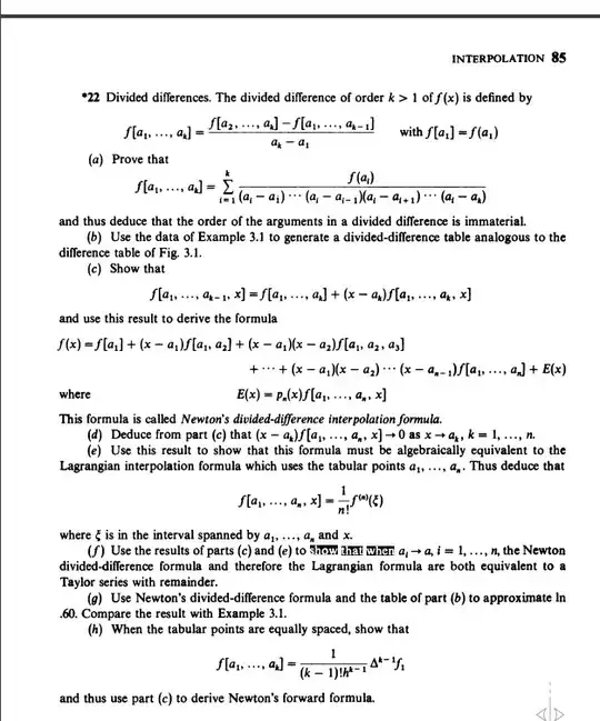
By algebraically equivalent in this case, the author refers to the fact that the Newton and Lagrange interpolating polynomials are identical, even though they are formed in different ways. The equivalence of these two polynomials follows from the fact that there is a unique polynomial of degree $n-1$ that interpolates the $n$ tabular points $\left\{a_{1},\ldots,a_{n}\right\}$.
The theoretical distinction between the Newton and Lagrange interpolating polynomials is that they are constructed using different basis functions. Suppose we have the tabular points $\left\{x_{0},\ldots,x_{n}\right\}$. The Newton basis for $P_{n}$ consists of the polynomials
\begin{equation*}
q_{j}(x) = \prod_{k=0}^{j-1}{(x-x_{k})}
\end{equation*}
with $q_{0}(x) = 1$. The Lagrange basis for $P_{n}$ consists of the polynomials
\begin{equation*}
\ell_{j}(x) = \prod_{\substack{k = 0\\ k\neq j}}^{n}{\frac{x-x_{k}}{x_{j}-x_{k}}}.
\end{equation*}
The Newton interpolating polynomial, constructed from the Newton basis, is
\begin{equation*}
p_{n}(x) = \sum_{j=0}^{n}{c_{j}q_{j}(x)}
\end{equation*}
where the $c_{j}$ are obtained from
\begin{equation*}
\left(\begin{array}{ccccc}
1 & 0 & 0 & \cdots & 0\\
1 & (x_{1}-x_{0}) & 0 & \cdots & 0\\
\vdots & \vdots & \vdots & \ddots & \vdots\\
1 & (x_{n}-x_{0}) & (x_{n}-x_{0})(x_{n}-x_{1}) & \cdots & \prod_{j=0}^{n-1}{(x_{n}-x_{j})}
\end{array}\right)\left(\begin{array}{c}
c_{0}\\
c_{1}\\
c_{2}\\
\vdots\\
c_{n}
\end{array}\right) = \left(\begin{array}{c}
f(x_{0})\\
f(x_{1})\\
f(x_{2})\\
\vdots\\
f(x_{n})
\end{array}\right).
\end{equation*}
Here is where the benefit of the Newton basis over, say, the monomial basis for the interpolating polynomial is apparent--this system is triangular, and easy to solve numerically.
On the other hand, the Lagrange interpolating polynomial is given by
\begin{equation*}
p_{n}(x) = \sum_{k=0}^{n}{c_{k}\ell_{k}(x)}.
\end{equation*}
By design, when $x = x_{j}$ all the terms vanish beside the $k = j$ term, where we find $p_{n}(x_{j}) = c_{j}\ell_{j}(x_{j}) = c_{j}$, so the coefficients obey
\begin{equation*}
\left(\begin{array}{ccccc}
1 & 0 & 0 & \cdots & 0\\
0 & 1 & 0 & \cdots & 0\\
\vdots & \vdots & \vdots & \ddots & \vdots\\
0 & 0 & 0 & \cdots & 1
\end{array}\right)
\left(\begin{array}{c}
c_{0}\\
c_{1}\\
c_{2}\\
\vdots\\
c_{n}
\end{array}\right) = \left(\begin{array}{c}
f(x_{0})\\
f(x_{1})\\
f(x_{2})\\
\vdots\\
f(x_{n})
\end{array}\right).
\end{equation*}
which is even easier to solve.
Now, to actually approach part (e) of the problem above, notice that $E(a_{k}) = 0$ for $k = 1,\ldots,n$.
