Minimizing linear least squares using Lagrangian $L(\mathbf{x}, \lambda) = f(\mathbf{x}) + \lambda (\mathbf{x}^T \mathbf{x} - 1)$

Question

Section 4.5 Example: Linear Least Squares of the textbook Deep Learning by Goodfellow, Bengio, and Courville, says the following:

Suppose we want to find the value of $\mathbf{x}$ that minimizes

$$f(\mathbf{x}) = \dfrac{1}{2}||\mathbf{A} \mathbf{x} - \mathbf{b}||_2^2 \tag{4.21}$$

Specialized linear algebra algorithms can solve this problem efficiently; however, we can also explore how to solve it using gradient-based optimization as a simple example of how these techniques work.

First, we need to obtain the gradient:

$$\nabla_{\mathbf{x}} f(\mathbf{x}) = \mathbf{A}^T (\mathbf{A}\mathbf{x} - \mathbf{b}) = \mathbf{A}^T \mathbf{A} \mathbf{x} - \mathbf{A}^T \mathbf{b} \tag{4.22}$$

We can then follow this gradient downhill, taking small steps. See algorithm 4.1 for details.

---

Algorithm 4.1 An algorithm to minimise $f(\mathbf{x}) = \dfrac{1}{2}||\mathbf{A} \mathbf{x} - \mathbf{b}||_2^2$ with respect to $\mathbf{x}$ using gradient descent, starting form an arbitrary value of $\mathbf{x}$.

---

Set the step size ($\epsilon$) and tolerance ($\delta$) to small, positive numbers.

while $||\mathbf{A}^T \mathbf{A} \mathbf{x} - \mathbf{A}^T \mathbf{b}||_2 > \delta$ do

$\ \ \ \mathbf{x} \leftarrow \mathbf{x} - \epsilon(\mathbf{A}^T \mathbf{A} \mathbf{x} - \mathbf{A}^T \mathbf{b})$

end while

---

One can also solve this problem using Newton's method. In this case, because the true function is quadratic, the quadratic approximation employed by Newton's method is exact, and the algorithm converges to the global minimum in a single step.

Now suppose we wish to minimize the same function, but subject to the constraint $\mathbf{x}^T \mathbf{x} \le 1$. To do so, we introduce the Lagrangian

$$L(\mathbf{x}, \lambda) = f(\mathbf{x}) + \lambda (\mathbf{x}^T \mathbf{x} - 1). \tag{4.23}$$

We can now solve the problem

$$\min_{x} \max_{\lambda, \lambda \ge 0} L(\mathbf{x}, \lambda). \tag{4.24}$$

The smallest-norm solution to the unconstrained least-squares problem may be found using the Moore-Penrose pseudoinverse: $\mathbf{x} = \mathbf{A}^+ \mathbf{b}$. If this point is feasible, then it is the solution to the constrained problem. Otherwise, we must find a solution where the constraint is active. By differentiating the Lagrangian with respect to $\mathbf{x}$, we obtain the equation

$$\mathbf{A}^T \mathbf{A} \mathbf{x} - \mathbf{A}^T \mathbf{b} + 2 \lambda \mathbf{x} = 0 \tag{4.25}$$

This tells us that the solution will take the form

$$\mathbf{x} = (\mathbf{A}^T \mathbf{A} + 2 \lambda \mathbf{I})^{-1} \mathbf{A}^T \mathbf{b} \tag{4.26}$$

The magnitude $\lambda$ must be chosen such that the result obeys the constraints. We can find this value by performing gradient ancient on $\lambda$. To do so, observe

$$\dfrac{\partial}{\partial{\lambda}} L(\mathbf{x}, \lambda) = \mathbf{x}^T \mathbf{x} - 1 \tag{4.27}$$

When the norm of $\mathbf{x}$ exceeds $1$, this derivative is positive, so to follow the derivative uphill and increase the Lagrangian with respect to $\lambda$, we increase $\lambda$. Because the coefficient on the $\mathbf{x}^T \mathbf{x}$ penalty has increased, solving the linear equation for $\mathbf{x}$ will now yield a solution with a smaller norm. The process of solving the linear equation and adjusting $\lambda$ continues until $\mathbf{x}$ has the correct norm and the derivative is $0$.

I've been wondering why the Lagrangian was chosen to take the form $L(\mathbf{x}, \lambda) = f(\mathbf{x}) + \lambda (\mathbf{x}^T \mathbf{x} - 1)$? Given the expression, it was obviously constructed this way intentionally, but I wonder what the reasoning was for using this Lagrangian?

I would appreciate it if people would please take the time to clarify this.

---

EDIT:

My understanding is that the term $\lambda (\mathbf{x}^T \mathbf{x} - 1)$ in $L(\mathbf{x}, \lambda) = f(\mathbf{x}) + \lambda (\mathbf{x}^T \mathbf{x} - 1)$ is the penalty. So the question is really one that revolves around penalties, and why the penalty $\lambda (\mathbf{x}^T \mathbf{x} - 1)$ was chosen for $f(\mathbf{x})$. So I think part of what I am misunderstanding here is the concept of penalties.

Answer 1

Update Version

It can be interpreted as follows by using the saddle-point property or the strong max-min property.

We want to solve the following convex optimization problem: $$\min_{x\in \mathbb{R}^n, \ x^Tx \le 1} \tfrac{1}{2}(Ax-b)^T(Ax-b). \tag{1}$$ If $(A^{+}b)^TA^{+}b\le 1$, clearly $x_0 = A^{+}b$ is the solution where $A^{+}$ is the Moore-Penrose inverse. In the following, we assume that $(A^{+}b)^TA^{+}b > 1$.

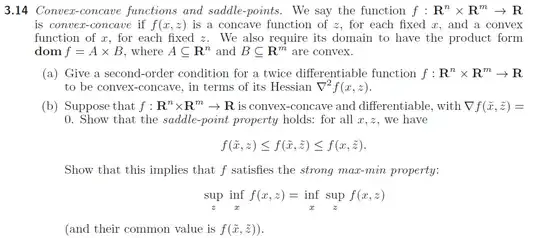
Denote $f(x) = \tfrac{1}{2}(Ax-b)^T(Ax-b)$. First, clearly, we have \begin{align} \sup_{\lambda \ge 0} [f(x) + \lambda (x^Tx - 1)] = \left\{\begin{array}{cc} f(x) & x^Tx \le 1 \\[3pt] +\infty & x^Tx > 1. \end{array} \right. \tag{2} \end{align} Thus, we have $$\min_{x\in \mathbb{R}^n, \ x^Tx \le 1} f(x) = \min_{x\in \mathbb{R}^n} \sup_{\lambda \ge 0} [f(x) + \lambda (x^Tx - 1)]. \tag{3}$$ Denote $L(x, \lambda) = f(x) + \lambda (x^Tx - 1)$. Clearly, $L(x, \lambda)$ is a convex function of $x$ on $\mathbb{R}^n$ for each fixed $\lambda \ge 0$, and a concave (indeed, affine) function of $\lambda$ on $[0, +\infty)$ for each fixed $x\in \mathbb{R}^n$. From exercise 3.14 in 1 (page 115), if there exists $(x^\ast, \lambda^\ast)$ with $\lambda^\ast \ge 0$ such that $\nabla L(x^\ast, \lambda^\ast) = 0$ where \begin{align} \nabla L(x, \lambda) = \left( \begin{array}{c} \frac{\partial L}{\partial x} \\[5pt] \frac{\partial L}{\partial \lambda} \\ \end{array} \right) = \left( \begin{array}{c} (A^TA + 2\lambda I)x - A^Tb \\[4pt] x^Tx - 1 \\ \end{array} \right), \tag{4} \end{align} then we have \begin{align} &\min_{x\in \mathbb{R}^n} \sup_{\lambda \ge 0} L(x, \lambda) = \sup_{\lambda \ge 0} \min_{x\in \mathbb{R}^n} L(x, \lambda) = L(x^\ast, \lambda^\ast) = f(x^\ast). \tag{5} \end{align} From (3) and (5), $x^\ast$ is the solution to the problem (1). As a result, any $(x^\ast, \lambda^\ast)$ with $\lambda^\ast \ge 0$ satisfying $\nabla L(x^\ast, \lambda^\ast) = 0$ gives the solution $x^\ast$ to the problem of (1).

Thus, we turn to solve the system of equations $\nabla L(x, \lambda) = 0$. To this end, we give the following result (the proof is given later):

Fact 1: If $(A^{+}b)^TA^{+}b > 1$, then there exists $\lambda^\ast > 0$ and \begin{align} x^\ast = (A^TA + 2\lambda^\ast I)^{-1}A^Tb \tag{6} \end{align} such that $(x^\ast)^T x^\ast = 1$. As a result, $\nabla L(x^\ast, \lambda^\ast) = 0$.

From Fact 1, we need to find $\lambda > 0$ such that $x = (A^TA + 2\lambda I)^{-1}A^Tb$ satisfying $x^Tx = 1$, equivalently, we need to find $\lambda > 0$ such that $g(\lambda) = 0$ where $$g(\lambda) = [(A^TA + 2\lambda I)^{-1}A^Tb]^T[(A^TA + 2\lambda I)^{-1}A^Tb] - 1.$$

References

1 Boyd and Vandenberghe, "Convex optimization". http://web.stanford.edu/~boyd/cvxbook/bv_cvxbook.pdf

exercise 3.14 (page 115)

[2] https://en.wikipedia.org/wiki/Moore%E2%80%93Penrose_inverse

$\phantom{2}$

Proof of Fact 1: For $\lambda > 0$, let $$g(\lambda) = [(A^TA + 2\lambda I)^{-1}A^Tb]^T[(A^TA + 2\lambda I)^{-1}A^Tb] - 1.$$ Clearly, $g(+\infty) = - 1$. By using the property of the Moore-Penrose inverse [2] $$A^{+} = \lim_{\delta \searrow 0} (A^TA + \delta I)^{-1}A^T,$$ we have $\lim\limits_{\lambda \searrow 0} g(\lambda) = (A^{+}b)^TA^{+}b - 1 > 0$. Thus, there exists $\lambda^\ast > 0$ such that $g(\lambda^\ast) = 0$. The desired result follows.

Answer 2

Having the sufficient regularity on $f(x), g(x)$, the Lagrangian stated as

$$ L(x,\lambda) = f(x)+\lambda g(x) $$

is used to determine the stationary points of

$$ \min(\max) f(x)\ \ \ \text{s. t.}\ \ \ g(x) = 0 $$

those points are the solutions for

$$ \nabla L = \cases{\partial_x f(x) +\lambda\partial_x g(x)=0\\ g(x)=0} $$

In the present case we have $g(x) = x^{\dagger}x\le 1$ then to handle this restriction with the lagrangian method, as $g(x)$ is no more an equation, we need to introduce a slack variable to transform the inequality into an equation so we augment the lagrangian to

$$ L(x,\lambda,\epsilon) = f(x) +\lambda(x^{\dagger}x-1+\epsilon^2) $$

and the stationary conditions are now

$$ \nabla L = \cases{A^{\dagger}(A x-b) +2\lambda x=0\\ x^{\dagger}x-1+\epsilon^2=0\\ \lambda\epsilon=0} $$

here, the last condition $\lambda\epsilon=0$ tell us that if $\lambda \ne 0$ the stationary point is internal/external to the set $x^{\dagger}x\lt1$ and if $\epsilon = 0$ the stationary point is at the boundary, or in $x^{\dagger}x=1$ then if the solution for

$$ A^{\dagger}(A \bar x-b)=0 $$

is such that

$$ \bar x^{\dagger}\bar x\lt 1 $$

we are done because $A^{\dagger}A\ge 0$ otherwise we should follow with

$$ \min(\max)f(x)\ \ \ \text{s. t.}\ \ \ x^{\dagger} x= 1 $$

NOTE

Now supposing $A$ is $m\times n$ with $m\ge n$ considering $U, V$ such that

$$ A = U\Sigma V^{\dagger},\ \ U^{\dagger}U=I,\ \ V^{\dagger}V = V V^{\dagger}=I $$

with

$$ \Sigma = \mbox{diag}\left(\sigma_1,\cdots,\sigma_n\right),\ \ \ \sigma_1\ge\cdots\ge \sigma_n\ge 0 $$

we have the equivalent problem

$$ \min ||\Sigma y-c||^2\ \ \text{s. t.}\ \ \ ||y||^2_2=1,\ \ \{y = V^{\dagger}x,\ c=U^{\dagger}b\} $$

with lagrangian

$$ L(y,\lambda) = ||\Sigma y-c||^2_2+\lambda(||y||_2^2-1) $$

with

$$ \left(\Sigma^2+\lambda I\right)\bar y = \Sigma c $$

and

$$ \bar y_k = \frac{\sigma_kc_k}{\sigma_k^2+\lambda} $$

and after substitution

$$ \sum_{k=1}^n\left(\frac{\sigma_kc_k}{\sigma_k^2+\lambda}\right)^2-1=0 $$

here $\lambda^*$ can be obtained with an iterative method like Newton's. Follows a MATHEMATICA script which handles the $\lambda=0$(internal solution) and $\epsilon=0$ (boundary solution) cases.

m = 5;
n = 3;
A = RandomReal[{-1, 1}, {m, n}];
b = RandomReal[{-1, 1}, m];
X = Table[Subscript[x, k], {k, 1, n}];
solx = Solve[Transpose[A].(A.X - b) == 0, X];
fact = X.X < 1 /. solx;
If[fact[[1]], Print["Internal solution"]; Print[X /. solx], Print["Boundary Solution"]]
If[Not[fact[[1]]], {U, Sigma, V} = SingularValueDecomposition[A];
c = Transpose[U].b;
sigma = Join[Table[Sigma[[k, k]], {k, 1, n}], Table[0, {m - n}]];
y = Table[sigma[[k]] c[[k]]/(sigma[[k]]^2 + lambda), {k, 1, m}];
sols = Quiet@Solve[y.y == 1, lambda, Reals];
y0 = y /. sols // N;
X0 = Union[Table[V.Take[y0[[k]], {1, n}], {k, 1, Length[y0]}]]]

Answer 3

When we talk about neural networks the large weights size can be a root cause of an unstable learning process. To prevent the increasing of the weights magnitude some constraint can be imposed. Popular choice is to use the max-norm constraint of all weights in the layer: $\mathbf{x}^T\mathbf{x} < c$.

Here is the citation from the popular paper Dropout: A Simple Way to Prevent Neural Networks from Overfitting: ...Though large momentum and learning rate speed up learning, they sometimes cause thenetwork weights to grow very large. To prevent this, we can use max-norm regularization.This constrains the norm of the vector of incoming weights at each hidden unit to be boundby a constant c...