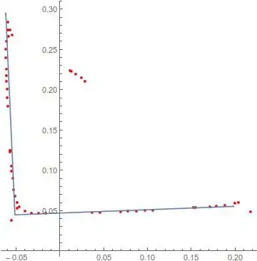
2

I have the convex hull of the corner of a building in 2D and I am trying to fit 2 perpendicular lines to the set of points on that hull to get me the orientation of the corner. I have a solution but its not useful for cases where one of the lines passes through the origin. Please let me know if any of the derivations aren't clear, I have only included the key results for the sake of being concise but can add more.

Say I have 2 sets of 2D points $\mathcal{X}_1$ and $\mathcal{X}_2$ belonging to line $l_1: \mathbf{x}^t\mathbf{n}=1$ and $l_2: \mathbf{x}^t\mathbf{Rn}/\alpha=1$ where $\mathbf{R}$ is a 90 degrees rotation matrix. This means that the distance of the line from the origin is given by one over the magnitude of $\mathbf{n}$.

Solution 1:

I can formulate a cost function:

$C = ||\mathcal{X}_1\mathbf{n}-\mathbf{1}_1||_2^2+||\mathcal{X}_2\mathbf{Rn}/\alpha - \mathbf{1}_2||_2^2$

where $\mathbf{1}_i$ is a vector of 1s with length equal to the number of points in set $i$

I can solve this equation easily giving:

$\mathbf{n} = \mathcal{X}_1^+\mathbf{1}_1$

$\alpha = ||\mathcal{X}_2\mathbf{Rn}||_1/N_2$

where $N_2$ is the number of points in set 2.

Firstly, I find it curious that the solution for $\mathbf{n}$ does not depend on any of the points in set 2, but also as mentioned, for a line that passes through the origin the answer is difficult to compute.

Solution 2

Instead, if I formulate the lines as $l_1: \mathbf{x}^t\mathbf{n}=d_1$ and $l_2: \mathbf{x}^t\mathbf{Rn}=d_2$ but this time constrain $\mathbf{n}$ to be a unit vector I can write my cost function using a lagrange multiplier to keep the constraint:

$C = ||\mathcal{X}_1\mathbf{n}-\mathbf{d}_1||_2^2+||\mathcal{X}_2\mathbf{Rn} - \mathbf{d}_2||_2^2 + \lambda(\mathbf{n^Tn}-1)$

This solution I am having trouble getting to a solution for - perhaps I am missing a constraint? Anyway if I differentiate with respect to $\mathbf{n}$ and set to 0 I get the following:

$(\mathcal{X}_1^T\mathcal{X}_1 + \mathbf{R}^T\mathcal{X}_2^T\mathcal{X_2}\mathbf{R} + \lambda\mathbf{I})\mathbf{n}=\mathcal{X}_1\mathbf{d}_1 + \mathbf{R}^T\mathcal{X}_2^T\mathbf{d}_2$

differentiating with respect to $\mathbf{d}_1$ and setting to 0 (noting that $\mathbf{d}_i=d_i\mathbf{1}_i$ and hence differentiating with respect to either the vector or scalar version and setting to 0 is equivalent)

I get $\mathbf{d}_1 = \mathcal{X}_1\mathbf{n}$ and similarly $\mathbf{d}_2 = \mathcal{X}_2\mathbf{Rn}$. First off this seems odd as it is an exact solution assuming no noise, but also when I substitute this to above everything cancels to give me $\lambda\mathbf{n}=0$ and I have no idea where to go from here.

Any help in how to get solution 2 making use of Lagrange multipliers would be grand - I have tried looking at formulating the problem in homogenous coordinates and am in the process of seeing whether that would work, but I a confused as to why the above gives no clear solution (or where my errors might be).

EDIT:

As requested in the comments here is a link to 4 different sets of sample data

For context, the purpose of this task is that I have some 3D data of the corner of a building and I am trying to work out the corner planes to align it with a coordinate axis. I have aligned the ground plane with a principal axis and then collapsed the points into 2D (effectively getting a plan view). Finally, to get the data presented I kept taking convex hulls until I had at least 50 points with a certain separation.

The data is unlabelled, and the process assigns points to a line based on proximity, although arguably a better classification scheme is likely possible since I know that it will be a corner.

EDIT 2

To clarify my question isn't how to find a solution to the problem - I already have one, my question is why solution 2 using Lagrange multipliers doesn't lead to a straightforward solution despite the almost trivial difference in formulation between Solution 1 and Solution 2.
falcoso
  • 121
  • Regarding Solution 2 have a look at https://math.stackexchange.com/questions/3524690/minimizing-linear-least-squares-using-lagrangian-l-mathbfx-lambda-f-ma/3537713#3537713 – Cesareo Feb 10 '20 at 12:33
  • So does that mean when the problem is formulated as in Solution 2, there is no closed-form solution? – falcoso Feb 10 '20 at 16:22
  • I also still don't understand why Solution 1 doesn't depend on the points in set 2 for calculating n – falcoso Feb 10 '20 at 17:29
  • @falcoso. I could propose a solution without iteration, without initial guess. The general principles are shown in : https://fr.scribd.com/doc/14819165/Regressions-coniques-quadriques-circulaire-spherique and https://fr.scribd.com/doc/14674814/Regressions-et-equations-integrales . But the particular case of two straight lines is not specifically treated in those papers. A couple of years ago I successfully used this method in a few cases of fitting two straight lines to scattered data. Would you mind to post at least an example of your data in order to check if it is convenient for you. – JJacquelin Feb 11 '20 at 13:47
  • have added data as requested – falcoso Feb 11 '20 at 16:19
  • @falcoso. The added data is very usefull to clarify the scope of the problem. Just by inspection the outliers points and sometimes more than two "linear" segments are not favourable to the non-iterative method. Sorry I think that the non-iterative method is not convenient for your problem. The method propoed by Cesareo is better in this case. – JJacquelin Feb 12 '20 at 16:01
  • Please see edit 2 to actually understand what I am asking - I have a solution and am not interested in solving it for my specific data set, I'm just simply trying to understand why a trivial difference in the problem formulation leads to a closed-form solution and the other one doesn't – falcoso Feb 13 '20 at 12:06

2 Answers2

0

Calling

$$ g_1(x,y) = y-y_0-m(x-x_0)\\ g_2(x,y) = y-y_0+\frac 1m(x-x_0) $$

and $T_1, T_2$ the data sets, we can formulate the minimization problem

$$ \min_{x_0,y_0,m}\left(\sum_{p_k\in T_1}g_1(p_k)^2+\sum_{p_k\in T_2}g_2(p_k)^2\right) $$

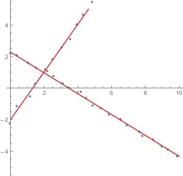
Follows a MATHEMATICA script to perform the calculations

Data preparation

g1[x_, y_] := y - y0 - m (x - x0)
g2[x_, y_] := y - y0 + 1/m (x - x0)
m = 1.5;
x0 = 2; y0 = 1; e = 0.2;
T1 = Table[{x + RandomReal[{-e, e}], y0 + m (x + RandomReal[{-e, e}] - x0)}, {x, 0, 10, 1/2}]
T2 = Table[{x + RandomReal[{-e, e}], y0 - 1/m (x + RandomReal[{-e, e}] - x0)}, {x, 0, 10, 1/2}]

Data processing

Clear[x0, y0, m]
f = Sum[g1[First[T1[[k]]], Last[T1[[k]]]]^2, {k, 1, Length[T1]}] + Sum[g2[First[T2[[k]]], Last[T2[[k]]]]^2, {k, 1, Length[T2]}];
sol = Minimize[f, {x0, y0, m}]
gr1 = ListPlot[T1];
gr2 = ListPlot[T2];
gr3 = ContourPlot[(g1[x, y] /. sol[[2]]) == 0, {x, 0, 10}, {y, -5, 5},
ContourStyle -> Red];
gr4 = ContourPlot[(g2[x, y] /. sol[[2]]) == 0, {x, 0, 10}, {y, -5, 5},
ContourStyle -> Red];
Show[gr1, gr2, gr3, gr4, PlotRange -> All, AspectRatio -> 1.6]

enter image description here

NOTE

Considering the furnished data with the sets $T_1, T_2$ mixed, the algorithm is as follows. Given a corner defined by

$$ p = \Lambda(p_0,\vec v,\lambda_1,\lambda_2) = \cases{p_0+\lambda_1\vec v\\ p_0+\lambda_2\vec v^{\top}},\ \ \ \{\lambda_1 \ge 0, \lambda_2 \ge 0, \vec v\cdot \vec v^{\top} = 0,\ ||\vec v||= 1\} $$

we calculate for each data point $p_k$ the minimum euclidean distance to $\Lambda(p_0,\vec v,\lambda_1,\lambda_2)$ which is $\left|\Lambda(p_0,\vec v,\lambda_1^k,\lambda_2^k)-p_k\right|$ and after that we minimize

$$ f(p_0,\vec v)=\sum_{k=1}^n\left|\Lambda(p_0,\vec v,\lambda_1^k,\lambda_2^k)-p_k\right| $$

The optimization MATHEMATICA script below implements this algorithm.

Clear[dist]
dist[vx_?NumericQ, vy_?NumericQ, px_?NumericQ, py_?NumericQ, pk_]:= Module[{lambda, d1,d2, v1 = {vx, vy}, v2 = {vy, -vx}, p0 = {px, py}},
lambda = -v1.(p0 - pk)/(v1.v1); 
If[lambda > 0, d1 = Sqrt[(p0 - pk + lambda v1).(p0 - pk + lambda v1)], 
d1 = Sqrt[(p0 - pk).(p0 - pk)]]; 
lambda = -v2.(p0 - pk)/(v2.v2); 
If[lambda > 0, d2 = Sqrt[(p0 - pk + lambda v2).(p0 - pk + lambda v2)], 
d2 = Sqrt[(p0 - pk).(p0 - pk)]]; Return[Min[d1, d2]]
]
sol = NMinimize[{Sum[dist[vx, vy, px, py, data[[k]]], {k, 1, Length[data]}], vx^2 + vy^2 == 1, -0.3 < px < 0.2, 0 < py < 0.4}, {vx, vy, px, py}, Method -> "DifferentialEvolution"]

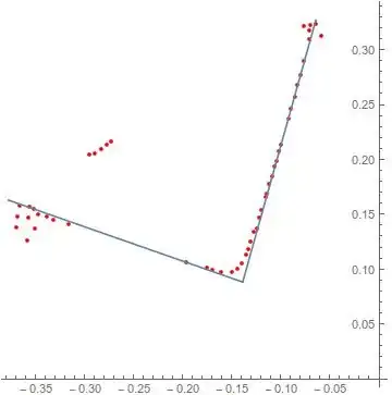
The results are shown below. Here data represents each of the furnished sets 1.txt, 2.txt, 3.txt,4.txt

enter image description here

enter image description here enter image description here enter image description here

Cesareo
  • 36,341
  • Does the fact that you have made this in Mathematica imply that the solution can't be found analytically? As mentioned under solution 1 I do have a closed-form method that works but am worried about it blowing up under lines that pass close to the origin – falcoso Feb 10 '20 at 16:40
  • Thinking about my model, the fitting process is much like a standard minimum square fit but with a nonlinear parameter which is $m$. Using the line parameterization as you proposed, with $\vec n = (n_x,n_y)$ and $\vec n^{\top} = (n_y,-n_x)$ in the case of Solution 1 a closed form solution can be found. Regarding Solution 2 I believe a closed form solution, should follow in a line shown in the previously cited reference. – Cesareo Feb 10 '20 at 19:08
  • In the reference though it uses an iterative solution to then find $\lambda$, which line are you referring to? – falcoso Feb 11 '20 at 11:32
  • Calling $$\phi(\lambda) = \sum_{k=1}^n\left(\frac{\sigma_kc_k}{\sigma_k^2+\lambda}\right)^2-1$$ we can use the Newton's iterative procedure to determine $\lambda^$ such that $\phi(\lambda^)=0$ as follows:

    $$ \lambda_{k+1}=\lambda_k-\frac{\phi(\lambda_k)}{\phi'(\lambda_k)} $$

    – Cesareo Feb 11 '20 at 13:35
  • As I could verify, the sample data has no separation for the line sets as suggested in the OP. This changes completely a successful approach. Why not adjusting orthogonal planes instead? This way we could use the data at it's full signification. From planes we can obtain orthogonal lines as well. – Cesareo Feb 12 '20 at 10:24
  • In the original 3d data some of the walls are very sparse, but the boundary is two consistent planes reducing to 2d and taking convex hulls puts points along that boundary no matter the view of the data – falcoso Feb 12 '20 at 12:58
  • @falcoso Please have a look at the attached note. – Cesareo Feb 12 '20 at 14:36
0

After two months I have finally found the closed-form solution and its actually blindingly obvious. It was inspired by closed-form solutions of point to point Iterative Closest Point (for which this problem was actually to try and help with the initial alignment for!)

So without further ado we have our cost function:

$C = ||\mathcal{X}_1\mathbf{n}-\mathbf{d_1}||_2^2+||\mathcal{X}_2\mathbf{Rn} - \mathbf{d_2}||_2^2 + \lambda(\mathbf{n}^T\mathbf{n}-1)\\$

If we subtract the mean from the set of points:

$C =\sum_{\hat{\mathbf{x}} \in \hat{\mathcal{X}}_1}(\mathbf{n}^T\hat{\mathbf{x}}+\mathbf{n}^T\mu_1-d_1)^2 + \sum_{\hat{\mathbf{x}} \in \hat{\mathcal{X}_2}}(\mathbf{n}^T\mathbf{R}^T\hat{\mathbf{x}}+\mathbf{n}^T\mathbf{R}^T\mu_2-d_2)^2 + \lambda(\mathbf{n}^T\mathbf{n}-1)$

$C= \sum_{\hat{\mathbf{x}} \in \hat{\mathcal{X}}_1}(\mathbf{n}^T\hat{\mathbf{x}}-d'_1)^2 + \sum_{\hat{\mathbf{x}} \in \hat{\mathcal{X}_2}}(\mathbf{n}^T\mathbf{R}^T\hat{\mathbf{x}}-d'_2)^2 + \lambda(\mathbf{n}^T\mathbf{n}-1) \\$

Expanding this out and noting that the mean of $\hat{\mathbf{x}}$ is 0: $ C = \mathbf{n}^T \left( \hat{\mathcal{X}}_1^T\hat{\mathcal{X}}_1 + \mathbf{R}^T\hat{\mathcal{X}}_2^T\hat{\mathcal{X}}_2\mathbf{R} + \lambda\mathbf{I} \right)\mathbf{n} -2\mathbf{n}^T\left( d'_1\sum_{\hat{\mathbf{x}} \in \hat{\mathcal{X}}_1}\hat{\mathbf{x}} + d'_2\sum_{\hat{\mathbf{x}} \in \hat{\mathcal{X}}_2}\hat{\mathbf{x}} \right) + N_1 {d'}_1^2 + N_2 {d'}_2^2 $

$ C = \mathbf{n}^T \left( \hat{\mathcal{X}}_1^T\hat{\mathcal{X}}_1 + \mathbf{R}^T\hat{\mathcal{X}}_2^T\hat{\mathcal{X}}_2\mathbf{R} + \lambda\mathbf{I} \right)\mathbf{n} + N_1 {d'}_1^2 + N_2 {d'}_2^2$

And therefore:

$ d_1 = \frac{1}{N_1}\mathbf{n}^T\sum_{\mathbf{x} \in \mathcal{X}_1}\mathbf{x}$

$ d_2 = \frac{1}{N_2}\mathbf{n}^T\sum_{\mathbf{x} \in \mathcal{X}_2}\mathbf{x}$

$ \mathbf{n} = \text{E-vector w/ min. e-value of } \hat{\mathcal{X}}_1^T\hat{\mathcal{X}}_1 + \mathbf{R}^T\hat{\mathcal{X}}_2^T\hat{\mathcal{X}}_2\mathbf{R}$

falcoso
  • 121