Two Categorical Variables
Checking if two categorical variables are independent can be done with Chi-Squared test of independence.
This is a typical Chi-Square test: if we assume that two variables are independent, then the values of the contingency table for these variables should be distributed uniformly. And then we check how far away from uniform the actual values are.
There also exists a Crammer's V that is a measure of correlation that follows from this test
Example
Suppose we have two variables
- gender: male and female
- city: Blois and Tours
We observed the following data:
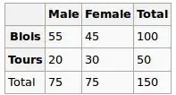
Are gender and city independent? Let's perform a Chi-Squred test. Null hypothesis: they are independent, Alternative hypothesis is that they are correlated in some way.
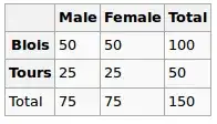
Under the Null hypothesis, we assume uniform distribution. So our expected values are the following
So we run the chi-squared test and the resulting p-value here can be seen as a measure of correlation between these two variables.
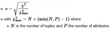
To compute Crammer's V we first find the normalizing factor chi-squared-max which is typically the size of the sample, divide the chi-square by it and take a square root
R
tbl = matrix(data=c(55, 45, 20, 30), nrow=2, ncol=2, byrow=T)
dimnames(tbl) = list(City=c('B', 'T'), Gender=c('M', 'F'))

chi2 = chisq.test(tbl, correct=F)
c(chi2$statistic, chi2$p.value)
Here the p value is 0.08 - quite small, but still not enough to reject the hypothesis of independence. So we can say that the "correlation" here is 0.08
We also compute V:
sqrt(chi2$statistic / sum(tbl))
And get 0.14 (the smaller v, the lower the correlation)
Consider another dataset
    Gender
City  M  F
   B 51 49
   T 24 26
For this, it would give the following
tbl = matrix(data=c(51, 49, 24, 26), nrow=2, ncol=2, byrow=T)
dimnames(tbl) = list(City=c('B', 'T'), Gender=c('M', 'F'))

chi2 = chisq.test(tbl, correct=F)
c(chi2$statistic, chi2$p.value)

sqrt(chi2$statistic / sum(tbl))
The p-value is 0.72 which is far closer to 1, and v is 0.03 - very close to 0
Categorical vs Numerical Variables
For this type we typically perform One-way ANOVA test: we calculate in-group variance and intra-group variance and then compare them.
Example
We want to study the relationship between absorbed fat from donuts vs the type of fat used to produce donuts (example is taken from here)
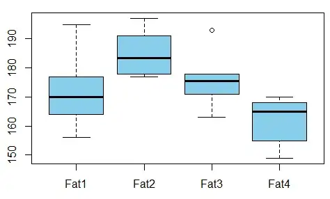
Is there any dependence between the variables?
For that we conduct ANOVA test and see that the p-value is just 0.007 - there's no correlation between these variables.
R
t1 = c(164, 172, 168, 177, 156, 195)
t2 = c(178, 191, 197, 182, 185, 177)
t3 = c(175, 193, 178, 171, 163, 176)
t4 = c(155, 166, 149, 164, 170, 168)

val = c(t1, t2, t3, t4)
fac = gl(n=4, k=6, labels=c('type1', 'type2', 'type3', 'type4'))

aov1 = aov(val ~ fac)
summary(aov1)
Output is
            Df Sum Sq Mean Sq F value  Pr(>F)
fac          3   1636   545.5   5.406 0.00688 **
Residuals   20   2018   100.9
---
Signif. codes:  0 ‘***’ 0.001 ‘**’ 0.01 ‘*’ 0.05 ‘.’ 0.1 ‘ ’ 1
So we can take the p-value as the measure of correlation here as well.
References