What's the idea?
I'm trying to embed the prime factorization problem into the form of a PUBO. To do so, let $p$ and $q$ be two real positive numbers. We can represent these two numbers as binary numbers, which itself can be represented as vectors, $\pmb{p}$ and $\pmb{q}$, where $\pmb{p}$ and $\pmb{q}$ both have $k$ elements. I define a new vector $\pmb{x}$ by concatenating $\pmb{p}$ and $\pmb{q}$ as follows:
$$p_i \in \{ 0,1\}$$ $$q_i \in \{ 0,1\}$$
$$ \pmb{x} = (p_1, \ldots, p_k, q_1, \ldots, q_{k})^T$$
Now I define the following matrix $Q$:
$$Q = \sigma_x \otimes \alpha$$
where $\alpha$ is a $k \times k$ matrix that its elements are defined like this:
$$\alpha_{ij} = 2^{2k - (i+j)}$$ and $$ \sigma_x = \begin{pmatrix} 0 & 1 \\ 1 & 0 \end{pmatrix} $$
This formulation, allows us to make $Q$ in a way that the product of numbers $p$ and $q$ is equal to the expression $\frac{1}{2}\pmb{x}^T Q \pmb{x}$:
$$\frac{1}{2}\pmb{x}^T Q \pmb{x} = pq$$
Now, I can also do this for $(pq)^2$:
$$\frac{1}{4}\pmb{x}^T Q \pmb{x}\pmb{x}^T Q \pmb{x} = (pq)^2$$
Now coming back to our original problem, we want to find the $p$ and $q$ so that:
$$pq = N$$
To do so, we can convert it into this optimization problem:
$$\min_{p,q} f(p,q) = \min_{p,q} (N-pq)^2$$
and using the PUBO form, we can convert $f$ to:
$$f(p,q) = N^2+ (pq)^2 - 2 N pq$$ $$f(p,q) = N^2+ \frac{1}{4}\pmb{x}^T Q \pmb{x}\pmb{x}^T Q \pmb{x} - N \pmb{x}^T Q \pmb{x}$$
Of course, this approach assumes that $\pmb{p}$ and $\pmb{q}$ have the same length of bits. To generalize this, we can simply move the separation point of vector $\pmb{x}$ from middle, one step at the time to get different lengths. This converts the complexity of the problem into:
$$O(N \log(N))$$
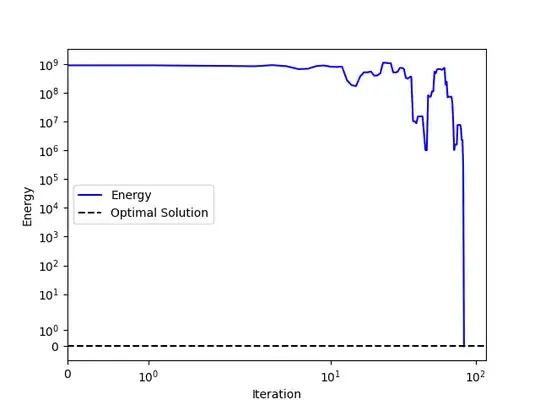
To solve this PUBO, I've tried simulated annealing and it works:
import numpy as np
import matplotlib.pyplot as plt
from tqdm import tqdm
def beta(N):
    pauli_x = np.array([[0, 1], [1, 0]])
def matrix_values(i, j):
    return 2**(2*N - (i+1)- (j+1))
matrix = np.fromfunction(matrix_values, (N, N))

# tensor product of pauli_x and matrix
matrix = np.kron(pauli_x, matrix)

return matrix


def preprocess(p, q):
    binary_p = bin(p)[2:]
    binary_q = bin(q)[2:]
# do a padding to make the length of binary_p and binary_q equal
if len(binary_p) < len(binary_q):
    binary_p = '0'*(len(binary_q) - len(binary_p)) + binary_p
elif len(binary_q) < len(binary_p):
    binary_q = '0'*(len(binary_p) - len(binary_q)) + binary_q

x = np.array(list(binary_p+binary_q), dtype=int)

return x


def simulated_annealing(B, pq, n_iterations=1000, T_start=100, T_end=0.1):
    # Initialize
    x = np.random.choice([0, 1], size=len(B))
    x[-1] = 1  # q must be odd
    x[len(x)//2] = 1  # p must be odd
T = T_start
energies = []
best_x = x.copy()
best_H = float('inf')

# Initial energy calculation
xBx = x @ B @ x
H = pq**2 + xBx**2 // 4 - pq * xBx

# Create tqdm progress bar
pbar = tqdm(range(n_iterations))

for i in pbar:
    # Generate new state
    j = np.random.randint(0, len(x))
    x_new = x.copy()
    x_new[j] = 1 - x_new[j]  # Flip the bit

    # Calculate energy difference efficiently
    delta_xBx = 0
    for k in range(len(x)):
        delta_xBx += B[j, k] * (x_new[j] - x[j]) * (x[k] + x_new[k])


    xBx_new = xBx + delta_xBx
    H_new = pq**2 + xBx_new**2 // 4 - pq * xBx_new

    # Calculate energy difference efficiently using vector operations
    delta_x = x_new - x
    delta_xBx = 2 * (delta_x @ B @ x) + (delta_x @ B @ delta_x)

    xBx_new = xBx + delta_xBx
    H_new = pq**2 + xBx_new**2 // 4 - pq * xBx_new

    # Calculate energy difference
    delta_H = (H_new - H) / pq**2

    # Decide whether to accept the new state
    if delta_H < 0 or np.random.random() < np.exp(-delta_H / T):
        x = x_new
        H = H_new
        xBx = xBx_new

    # Cool down
    T = T_start * (T_end / T_start) ** (i / (n_iterations - 1))
    energies.append(H)

    # Update best state
    if H < best_H:
        best_x = x.copy()
        best_H = H
    if best_H == 0:
        break
    # Update tqdm description with current best_H
    pbar.set_description(f"Best H: {best_H:.4e}")

energies = np.array(energies)

return best_x, best_H, energies


p , q = 241, 251
pq = p*q
L = (np.floor(np.log2(float(pq))).astype(int)) //2 + 1
B = beta(L)
x, H, energies = simulated_annealing(B, pq, n_iterations=10_000, T_start=1e-1, T_end=1e-5)
get back the values of p and q
p_o = int(''.join(map(str, x[:L])), 2)
q_o = int(''.join(map(str, x[L:])), 2)
print(H)
print(p_o, q_o)
plt.plot(energies, color='b', linestyle='-', label='Energy')
plt.yscale('symlog')
plt.xscale('symlog')
plt.xlabel('Iteration')
plt.ylabel('Energy')
plt.hlines(0,xmin=0, xmax=1.4len(energies), color='black', linestyle='--', label='Optimal Solution')
plt.xlim(0, 1.4len(energies))
plt.legend(loc = 'center left')
plt.show()
Note that my code assumes the same length of bits for both numbers, but as mentioned before, it can be generalized pretty easily. This code successfully factors the number 60491 to 241 and 251.
What's the catch?
The catch is that the simulated annealing is not a good way of optimization for large $N$. There are far better Ising machines for these types of tasks, but the problem is the fact that they are designed to work with QUBOs, not PUBOs. But now, I tell my suggestion:
We should be able to solve this using a modified version of the Simulated Bifurcation algorithm.
It is highly parallelizable, and it reaches to the solution in orders of magnitude less time. I also think there are tons of other optimizations in the embedding itself. Plus, I believe we should be able to combine this approach with classical algorithms such as Sieve of Eratosthenes. Please tell what you think about my approach. Any comment would be greatly appreciated.
