I want to do something like this:
For a single-qubit
- Apply Hadamard -> Time_evolution -> Phase_damping -> Hadamard -> Post-selection -> Get CFI(classical fisher info)
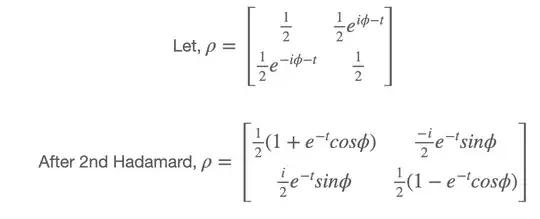
Density matrix after Phase_damping is: (You can see the e^-t added at the off-diagonal term) You can also see the density-matrix after the 2nd Hadamard gate.

However, I want to apply post-selection like this:

After that, I expect to get following (t/t2 -> t):

Is there any possible method to get that in pennylane?
I already worked for
- Generate quantum circuit that returns density-matrix after 2nd Hadamard gate
- Get that density-matrix from the quantum circuit above, operate post-selection calculation using numpy.
- Generate another quantum circuit with the result of the above density matrix
- Calculate Classical Fisher Information.
So, everything works fine But, I can't find the function which implement 'post-selection' kind of operate in pennylane. I wonder if there is any smarter way(I don't want to make quantum-circuit twice) to do that.
And here is code I worked for:
import pennylane as qml
from pennylane import numpy as np
import matplotlib.pyplot as plt
== Hamiltonain setup ==
Coeff_ham = [1]
Obs = [qml.PauliZ(0)]
Hamiltonian = qml.Hamiltonian(Coeff_ham, Obs)
dev = qml.device("default.mixed", wires = 1)
== gamma -> t ==
gamma = 0.5
t = -np.log( np.sqrt(1 - gamma))
== Define gammma ==
t = 0.0001
gamma_dephase = 1 - np.exp(-2 * t)
gamma_ps = 0.8
Stage_1: Generate dephase
@qml.qnode(dev)
def Dephase_circuit(phi):
    qml.Hadamard(wires=0)
# Time_evo t fixed as -phi/2
qml.ApproxTimeEvolution(Hamiltonian, -phi/2, 1)

qml.PhaseDamping(gamma_dephase, wires = 0)

qml.Hadamard(wires=0)

return qml.density_matrix(wires=0)


Stage_2: Post-selection
@qml.qnode(dev)
def Post_selection(phi):
    rho_dephase = Dephase_circuit(phi)
    Kraus_oper = np.array([ [np.sqrt(1-gamma_ps), 0], [0, 1] ])
rho_ps = (Kraus_oper @ rho_dephase @ Kraus_oper.conj().T) / (np.trace(Kraus_oper @ rho_dephase @ Kraus_oper.conj().T))
qml.QubitDensityMatrix(rho_ps, wires=0)

return qml.density_matrix(wires=0)


== Plot for CFI ==
N = 100
tau_CFI = np.linspace(-0.001, 6.2, N)
CFI_0 = np.zeros(N)
CFI_1 = np.zeros(N)
CFI_2 = np.zeros(N)
t = 0.0001
gamma_dephase = 1 - np.exp(-2 * t)

for i in range(len(tau_CFI)):
            CFI_0[i] = (qml.qinfo.transforms.classical_fisher(Post_selection)(tau_CFI[i]))
t = 0.01
gamma_dephase = 1 - np.exp(-2 * t)

for i in range(len(tau_CFI)):
            CFI_1[i] = (qml.qinfo.transforms.classical_fisher(Post_selection)(tau_CFI[i]))
t = 0.1
gamma_dephase = 1 - np.exp(-2 * t)

for i in range(len(tau_CFI)):
            CFI_2[i] = (qml.qinfo.transforms.classical_fisher(Post_selection)(tau_CFI[i]))
plt.plot(tau_CFI, CFI_0, label = '$t$ = 0.0001')
plt.plot(tau_CFI, CFI_1, label = '$t$ = 0.01')
plt.plot(tau_CFI, CFI_2, label = '$t$ = 0.1')
plt.title('Classical Fisher Information at near zero')
plt.title('Classical Fisher Information at $\gamma$ = 0.8')
plt.xlabel('Time')
plt.ylabel('CFI')
plt.legend()
plt.grid()
Thanks in advance.