What is the average euclidean distance between two points on the surface of a hypersphere of dimension $n$?

Question

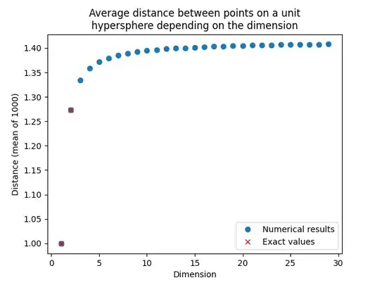
Take the surface of the unit hypersphere of dimension $n$: $$ S = \{x\in\mathbb{R}^n: \lVert x \rVert = 1\} $$ Given two uniformly sampled points on its surface, what is the expected distance between them? And how does the distance scale with the radius? To clarify, I'm asking about Euclidean distance, not along a great circle. This question already answers the question for great circles in any dimension. I made this numerical experiment, which might suggest that the limit is $\sqrt 2$:

Here is the code if you want to try it yourself:

import numpy as np
from scipy.spatial.distance import cdist
import matplotlib.pyplot as plt
def random_on_unit_hypersphere(dim: int, n: int = 1) -> np.ndarray:
    mean = np.zeros(dim)
    cov = np.identity(dim)
    result = np.random.multivariate_normal(mean, cov, size=n)
    norm = np.linalg.norm(result, axis=1)[:, None]
    return result / norm
fig, ax = plt.subplots()
ax.set(title='Average distance between points on a unit\nhypersphere depending on the dimension', 
       xlabel='Dimension', ylabel='Distance (mean of 1000)')
dims = np.arange(1, 30)
means = []
for dim in dims:
    # Randomize 1000 points uniformly on the hypersphere of dimension dim.
    points = random_on_hypersphere(dim, n=1000)
    # Get the matrix where distances[i, j] == np.linalg.norm(points[i] - points[j]).
    distances = cdist(points, points)
    # The matrix is symmetric, so only take the mean of the values from the upper triangle.
    upper_triangle_indices = np.triu_indices_from(distances, k=1)  # k=1 means 1 above the diagonal
    unique_distances = distances[upper_triangle_indices]
    means.append(np.mean(unique_distances))
ax.plot(dims, means, 'o', label='Numerical results')
ax.plot([1, 2], [1.0, 4/np.pi], 'x', color='red', label='Exact values')
ax.legend()
plt.show()

Answer 1

Here's a sketch of something that might work (mostly a long comment). Any two points on a sphere determine a great circle, and the distance you're interested in is a chord of that great circle.

Therefore, this problem can be reduced to studying distances on a circle with a non-uniform probability measure on the circle. The probability measure is based on the relative area of spherical caps on $\mathbb{S}^n$.

You'll find that as the dimension increases, all of the surface area of the sphere is concentrated about the equator of the sphere. This means that if the second point is chosen randomly, it's very likely to be perpendicular to your first point.

So, the expected distance should approach the distance between two perpendicular points on the circle, i.e., $\sqrt{2}$.

This is not a proof, but a sketch of how one might verify the $\sqrt{2}$ value that you found.

Answer 2

The result you found seems to be correct based on some basic results that are always true for Euclidean vectors.

The squared distance between two such vectors $\vec{v},\vec{w}\in\mathbb{R}^n$ is:

\begin{align*} ||\vec v-\vec w||^2 &= \langle \vec v-\vec w, \vec v-\vec w \rangle \\&= \vec v^2 + \vec w^2 -2\langle \vec v, \vec w\rangle \\&= \vec v^2 + \vec w^2 - 2||\vec v||\ ||\vec w|| \cos(\angle(\vec v,\vec w)) \end{align*}

Now in your case $\vec v^2 = \vec w^2 = 1$ and also $||\vec v||=||\vec w||=1$. So this immediately gives:

$$ ||\vec v-\vec w||^2 = 2-2\cos(\angle(\vec v,\vec w))\\ \Rightarrow ||\vec v-\vec w|| = \sqrt{2-2\cos(\angle(\vec v,\vec w))}, $$

Now we know that the expected value for this last expression is attained when $\cos(\angle(\vec v,\vec w))=0$, for a random collection of vectors in $\mathbb{R}^n$, because the mean for the cosine function is precisely 0. I understand however that in higher dimensions the angles between a random collection of vectors aren't uniformly distributed in the interval $[0, \pi]$ so this needs some more careful consideration, but hopefully this gives you a concrete direction on how to tackle this.

Answer 3

Without loss of generality we assume $R=1$. If $U$ and $U_1$ are independent and uniform on the unit sphere of the Euclidean space $R^n$ we are asked for the value of $E(\|U-U_1\|).$ Without loss of generality we may replace $U_1$ by $e_1=(1,0,\ldots,0).$ For computing the density of $\|U-e_1\|$ we consider $Z\sim N(0,I_n)$ and observe $U\sim Z/\|Z\|.$ We denote $Y^2=Z_2^2+\cdots+Z_n^2.$ Now $$\|U-e_1\|^2\sim 2\left(1-\frac{Z_1}{\sqrt{Z_1^2+Y^2}}\right).$$ The law of $V=\frac{Z_1^2}{Z_1^2+Y^2}$ is a beta distribution $\beta(1/2,(n-1)/2)$ with density on $(0,1)$ equal to $$v^{-1/2}(1-v)^{(n-3)/2})/B_n$$ with $B_n=B(1/2,(n-1)/2).$ Therefore the density of $W=\sqrt{V}$ on $(0,1)$ is $2(1-w^2)^{(n-3)/2})/B_n$ and the density of $T=Z_1/\sqrt{Z_1^2+Y^2}$ on $(-1,1)$ is $(1-t^2)^{(n-3)/2})/B_n.$ We are in position to compute $$E((2(1-T))^{1/2})=\frac{\sqrt{2}}{B_n} \int_{-1}^1(1-t)^{1/2}(1-t^2)^{(n-3)/2})dt$$ by the change of variable $s=(1-t)/2$ and obtaining $$E((2(1-T))^{1/2})=\frac{2^{n-1}}{B_n}B(n/2,(n-1)/2)\to \sqrt{2}$$ by Stirling formula, as predicted by previous contributors.