Invariance of Lyapunov exponents under diffeomorphisms

Question

I have a fundamental question about the behavior of Lyapunov exponents under smooth transformations.

Intuitively, I would expect that a chaotic system's Lyapunov exponents will not be preserved if, instead of measuring the system's state $\vec{x}$, one observes a transformed state $\vec{y}=g(x)$.

For example, if our dynamical system is described by $\dot{x}=\lambda x$, it will have one Lyapunov exponent of $\lambda$ because the solution is $x(t)=x_0e^{\lambda t}$ (I'll assume $x_0\geq 1$). If one considers $y=x^2$, this new variable will evolve according to $\dot{y}=2x\dot{x}=2\lambda y$ which corresponds to a system with Lyapunov exponent $2\lambda\neq\lambda$.

However, I am confused by this for two reasons.

1. It would seem that this conflicts with the common approach for computing Lyapunov exponents in practice. That approach is to (1) construct a high-dimensional state using time delays (by Taken's embedding theorem, this new state allows you to reconstruct your chaotic attractor up to diffeomorphism) and then (2) compute Lyapunov exponents using these new state vectors [1,2]. Why does this work? I would imagine that if your experimental apparatus only lets you measure the system state through some distorted "lens" (for example by observing $x^2$ instead of $x$) then the exponents you measure in this procedure would not correspond to the true ones.

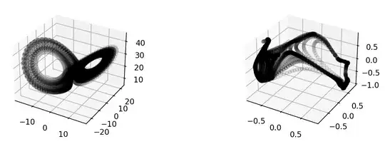
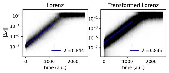
2. If I play around and use a (random) neural network to distort a Lorenz attractor and then compute Lyapunov exponents using the distorted state, I find the same exponents! It would appear that these transformations don't make a difference (as long as they are close to invertible).

These two points would seem to conflict with my simple example from above. What am I missing? The only fundamental difference to me is that in the example, the state is unbounded, while any system residing on a (strange) attractor is bounded. If this is issue is addressed in the literature, I'd be happy if someone could point me in the right direction.

---

---

Below, the results of my numerical experiment.

Left, Lorenz. Right, Lorenz after being fed through a random neural network.

Measured (top) exponents by tracking many close trajectories.

Answer 1

The fundamental difference between these two problems is, indeed, the fact that the system $\dot{x}=\lambda x$ is unbounded. The fact that the flows on the Lorenz attractor are bounded guarantees you that the Lyapunov exponents will not change if you transform the system by changing coordinates to $y = g(x)$ where $g$ is smooth and invertible.

For the single-dimensional case, the proof of this is not too challenging. Consider $\dot{x} = f(x)$ with $y = g(x)$ a smooth, invertible coordinate change. The Lyapunov exponents are defined as: $$ \lambda_x = \lim_{t\to\infty}\frac{1}{t}\ln\left|\frac{dx(t)}{dx(0)}\right| $$$$ \lambda_y = \lim_{t\to\infty}\frac{1}{t}\ln\left|\frac{dy(t)}{dy(0)}\right| $$

By the chain rule, $\dot{y} = g'(x)f(x)$. Hence, we can write: $$ \frac{dy(t)}{dy(0)} = \frac{g'(x(t))}{g'(x(0))}\frac{dx(t)}{dx(0)} $$

Since $g$ is invertible, we know that $g'$ is non-zero everywhere. Hence, we can take the logarithm of any of its flows: $$ \ln\left|\frac{dy(t)}{dy(0)}\right| = \ln|g'(x(t))| - \ln|g'(x(0))| + \ln\left|\frac{dx(t)}{dx(0)}\right| $$

Now, consider $$ \lambda_y = \lim_{t\to\infty}\frac{1}{t}\left(\ln|g'(x(t))| - \ln|g'(x(0))| + \ln\left|\frac{dx(t)}{dx(0)}\right|\right) $$

Since $g'(x(0))$ is a constant, the $\ln|g'(x(0))|$ term goes to zero. We are left with the following result: $$ \lambda_y = \lambda_x + \lim_{t\to\infty}\frac{1}{t}\ln|g'(x(t))| $$

When $x(t)$ is bounded away from zero and infinity, then $g'(x(t))$ is similarly bounded. Hence, the limit goes to zero, and you arrive at $\lambda_y = \lambda_x$.