Is a random variable always an identity mapping for continuous distributions?

Question

This seems like a dumb question, but surprisingly I have not been able to find a definitive answer.

Basic understanding:

• A random variable is a function which maps from the sample space to the real line, i.e. $X: \Omega \rightarrow \Bbb R$. The r.v. $X$ might map onto a subset of $\Bbb R$, depending on the situation.

• The pmf/pdf take as "input" real numbers $x \in Range(X)$ and assigns probabilities/densities to them...in other words, the domain of the pdf/pmf is the range of the r.v. $X$.

Discrete r.v.s

For discrete distributions, the sample space is often meaningful; it is the domain of the r.v. of that distribution. For example, if $X\sim Binomial(n, p)$, the sample space of outcomes is $\Omega = Domain(X) = \{(TTT...TT), (TTT...TH), \dots\}$ representing all possible n-tuples of "n" heads or tails. The r.v. X is then a "counting" function, as it maps from each outcome in this sample space (which is an n-tuple) to the number of heads (a real number). Here, X has a purpose.

Continuous r.v.s

For most continuous distributions I have come across, the random variable is itself is just the identity mapping.

• For the Normal, the "sample space" is $\Bbb R$. When $X \sim Normal(\mu, \sigma^2)$, the domain of pdf $f(x)$ if $\Bbb R$. So $X: \Bbb R \rightarrow \Bbb R$ is just an identity mapping.
• For the continuous uniform, the "sample space" is $\Bbb R$. Note that $f(x)$ here only has support on $[a, b]$, but is defined on $\Bbb R$, and thus the sample space is $\Bbb R$. Thus, $X: \Bbb R \rightarrow \Bbb R$ is once again an identity mapping.
• For the Beta, the "sample space" is $[0, 1]$, since the Beta is not defined elsewhere. Her, $X: [0, 1] \rightarrow [0, 1]$ is again an identity mapping.
• The same holds for the Exponential, Gamma, etc.

I have two questions:

1. Is my understanding correct for the continuous distributions I listed above?
2. Is this a property of all continuous random variables, or is this just the case for the distributions I have described?

Answer 1

Basic understanding:

The definition of a r.v. is always in the context of a probability space $(\Omega, \mathscr F, P)$, where $\mathscr F$ is a $\sigma$-algebra of subsets (called "events") of the sample space $\Omega$, and $P:\mathscr F\to[0,1]$ is a probability measure; i.e. $P(A)$ is defined only for events $A\in\mathscr F$.

A random variable is a function which maps from the sample space to the real line, i.e. $X: \Omega \rightarrow \Bbb R$. The r.v. $X$ might map onto a subset of $\Bbb R$, depending on the situation.

There is also a requirement that the function $X: \Omega \rightarrow \Bbb R$ must be measurable (i.e., for every Borel subset $B\subseteq\Bbb R$, the set $\{\omega\in\Omega: X(\omega)\in B\}$ must be in the $\sigma$-algebra $\mathscr F$.

The pmf/pdf take as "input" real numbers $x \in Range(X)$ and assigns probabilities/densities to them...in other words, the domain of the pdf/pmf is the range of the r.v. $X$.

Yes, except that the domain of definition of the p.d.f/p.m.f is typically extended to all of $\Bbb R$, taking them to be zero outside the range of $X$. (We're using "range" here to mean "image", not codomain.)

Discrete r.v.s

For discrete distributions, the sample space is often meaningful; it is the domain of the r.v. of that distribution. For example, if $X\sim Binomial(n, p)$, the sample space of outcomes is $\Omega = Domain(X) = \{(TTT...TT), (TTT...TH), \dots\}$ representing all possible n-tuples of "n" heads or tails. The r.v. X is then a "counting" function, as it maps from each outcome in this sample space (which is an n-tuple) to the number of heads (a real number). Here, X has a purpose.

The distribution of a r.v. does not determine its domain. For example, the Binomial distribution can arise as you've described; however, mathematically, we could certainly have $\Omega=\{0,1,...,n\}$, with $X(\omega)=\omega,$ and the exact same p.m.f.

Continuous r.v.s

For most continuous distributions I have come across, the random variable is itself is just the identity mapping.

Again, the distribution of a r.v. does not determine its domain, but if the domain is not specified then we can always take the probability space to be $(\Omega,\mathscr F, P)=(\Bbb R, \mathscr B({\Bbb R}),P)$, where $P()$ is defined by the p.d.f./p.m.f. (or more generally the c.d.f.), with $X$ the identity function.

For the continuous uniform, the "sample space" is $\Bbb R$. Note that $f(x)$ here only has support on $[a, b]$, but is defined on $\Bbb R$, and thus the sample space is $\Bbb R$. Thus, $X: \Bbb R \rightarrow \Bbb R$ is once again an identity mapping.

Consider the Uniform distribution on $[0,1]$. Here are two quite different models:

1. (identity map) $(\Omega,\mathscr F,P)=(\Bbb R,\mathscr B({\Bbb R}),P)$, where $X$ is the identity function on $\Bbb R$, with p.d.f. $f_X(x)=1_{x\in[0,1]}$ for all $x\in\Bbb R$. For any Borel subset of $\Bbb R$, we have $P(X\in B):=\int_{B}f_X(x)\,dx.$

2. (coin tosses as random digits) $(\Omega,\mathscr F,P)=(\{0,1\}^\infty,\mathscr B(\{0,1\}^\infty),P)$, where $P$ is the product measure on the Borel subsets of $\{0,1\}^\infty$, whose marginals are Uniform on $\{0,1\}$, and $X(\omega_1\omega_2...):=(0.\omega_1\omega_2...)_2.$
   This models a "thought experiment" whose outcome $\omega=(\omega_1,\omega_2,...)$ is the binary sequence resulting from tossing a fair "0-or-1" coin infinitely many times, and $X(\omega)$ is just that sequence read as a base-2 numeral (prefixed by "$0.$"). It can be shown that the distribution of $X$ is exactly Uniform on $[0,1]$.

More generally, we have the inverse probability integral transform theorem:

If $X$ is a r.v. whose c.d.f. is $F$, then the r.v. $F^{-1}(U)$ has the same distribution as $X$, where $F^{-1}$ is the generalized inverse of $F$ and $U$ is a r.v. with Uniform distribution on $[0,1]$.

Thus, if a r.v. with c.d.f. $F$ has unspecified domain, then the domain could be $[0,1]$, because the distribution can't be distinguished from that of r.v. $F^{-1}:\Omega\to\Bbb R$, where $(\Omega,\mathscr F,P)=([0,1],\mathscr B([0,1]),P)$ with Uniform distribution $P$.

Answer 2

I think I have an answer for question 2; the random variable is not an identity mapping for all continuous distributions.

The counterexample is as follows:

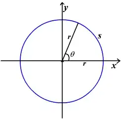
• Consider a unit circle centered at the origin as our sample space. Each "outcome" in our sample space is a pair $(x_1, x_2)$, where we have the restriction $x_1^2 + x_2^2 =1$. Let's call this $\Omega_{circle}$. It's a set, so it's a valid sample space.

• $\Omega_{circle}$ is an uncountably infinite set, so it can only be the sample space of a continuous distribution, not a discrete distribution.

• Let the r.v. $X$ measure the angle in radians of the point $(x_1, x_2) \in \Omega_{circle}$. Without loss of generality, assume we measure the angle anticlockwise from (1, 0) (see the picture below...normally we call this $\theta$ but here I'll call it $X$).

• Since $X$ measures the radians, we have $X: \Omega_{circle} \rightarrow (0, 2\pi]$. $X$ is a valid r.v. since it maps from the sample space to a subset of the real line.

• Let's define some sort of density function $f(x)$ on top of $X$...for simplicity, let's just use the uniform density, i.e. $f(x) = \frac{1}{2\pi}, { } \forall x \in Range(X)$, where $Range(X) = (0, 2\pi]$. We can easily see this is a valid density, since $f(x) \ge 0$ and $\int_{-\infty}^{\infty} f(x) \, dx = \int_0^{2\pi} f(x) \, dx = \int_0^{2\pi} \frac{1}{2\pi} \, dx = (\frac{1}{2\pi})(2\pi) = 1$

Thus, we have setup a continuous distribution where $X$ is not an identity mapping.

Answer 3

Your intuition is correct when we have exactly one random variable that we care about. This usually is not the case, however. For instance, we might have a sequence $(X_i)_i$ of i.i.d random variables. In this case, the natural sample space $\Omega$ is a product space with the probability measure being a product measure. For any individual random variable $X_i$ in this collection, the mapping $\omega \to X_i(\omega)$ is not an identity mapping but rather some sort of projection.

When we have want to model sequences of random variables with more complicated interdependencies, like martingales or Markov chains, the sample space can be far more complicated. However, there are known results like the Kolmogorov extension theorem which ensure that a sample space exists for pretty much any meaningful situation we want to model.