Joint probability of random variates

Question

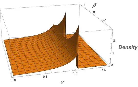
Let X and Y be two normally distributed variables with mean = 0 and variances $\sigma_x, \sigma_y$. I am interested in finding the joint probability distribution $P(\alpha,\beta)$ of two quantities given as:

$$\tan^2{\alpha} = X^2 + Y^2$$

and

$$\tan{\beta} = \frac{Y}{X}$$.

I have found the probabilities $P(\alpha)$ and $P(\beta)$. $P(\tan{\beta})$ is a Cauchy distribution with the scale parameter being the ratio of variances while $P(\tan^2{\alpha})$ is a generalized $\chi^2$ distribution as detailed here. I can then find $P(\alpha)$ and $P(\beta)$ through a change of variables. However, I am struggling to find $P(\alpha, \beta)$. I attempted using the conditional probability such that $$P(\alpha,\beta) = \frac{P(\alpha | \beta)}{ P(\beta)}$$ but without success. Is there some way to obtain the joint distribution?

One of the problems I am facing is that for the particular case of $\sigma_x = \sigma_y$, the distribution of $P(\alpha,\beta)$ should not have a dependency on $\beta$ as $P(\beta)$ is uniform. I cannot retrieve any joint distribution with such properties.

Edit1: Typo, X and Y are normally distributed.

Edit2: I think I found the solution. Following this post!

We know $A \sim N(0, \sigma_x)$ and $B \sim N(0, \sigma_y)$. We are interested in mapping $$(A,B) \rightarrow (\arctan{\sqrt{A^2 + B^2}},\arctan{\frac{B}{A}}) = (\alpha,\beta)$$ as \begin{equation*} \alpha = \arctan{\sqrt{a^2 + b^2}}, \beta = \arctan{\frac{b}{a}} \Rightarrow a = \cos(\beta)\tan(\alpha), b = \sin(\beta)\tan(\alpha) \end{equation*} The jacobian determinant can be computed as \begin{equation*} J = \begin{vmatrix} \frac{\partial a}{\partial \alpha} & \frac{\partial a}{\partial \beta} \\ \frac{\partial b}{\partial \alpha} & \frac{\partial b}{\partial \beta} \\ \end{vmatrix} = \begin{vmatrix} \frac{\cos(\beta)}{\cos^2(\alpha)} & -\sin(\beta)\tan(\alpha) \\ \frac{\sin(\beta)}{\cos^2(\alpha)} & \cos(\beta)\tan(\alpha) \\ \end{vmatrix} = \frac{\tan(\alpha)}{\cos^2(\alpha)} \end{equation*}

We can obtain $f(\alpha, \beta)$ from \begin{equation*} f_A(a) f_B(b) da db = \frac{1}{\sigma_x \sqrt{2\pi}} \exp{\frac{-a^2}{2\sigma_x^2}} \frac{1}{\sigma_y\sqrt{2\pi}} \exp{\frac{-b^2}{2\sigma_y^2}} dadb = \frac{1}{\sigma_y \sigma_x 2\pi} \exp{-\frac{\sigma_y^2a^2+\sigma_x^2 b^2}{2\sigma_x^2\sigma_y^2}} da db \end{equation*}

Focusing now on the term on the exponent we need to factorize $\sigma_y^2a^2+\sigma_x^2 b^2$ in terms of $a^2 + b^2 = \tan^2(\alpha)$ and $\frac{b}{a} = \tan(\beta)$. Multiplying and dividing the expression by $a^2$ and by $\frac{(a^2 + b^2)}{(a^2 + b^2)}$ we obtain for the \begin{equation*} \sigma_y^2a^2+\sigma_x^2 b^2 = (a^2 + b^2) \frac{a^2}{a^2 + b^2} (\sigma_y^2 + \frac{b^2}{a^2}\sigma_x^2) = \tan^2(\alpha) \cos^2(\beta)(\sigma_y + \tan^2(\beta)) \end{equation*} The final expression then yields \begin{equation*} f(\alpha,\beta) = \frac{1}{\sigma_y \sigma_x 2\pi} \exp{-\frac{\tan^2(\alpha) \cos^2(\beta)(\sigma_y^2 + \sigma_x^2\tan^2(\beta))}{2\sigma_x^2\sigma_y^2}} \frac{\tan(\alpha)}{\cos^2(\alpha)} \end{equation*}

The expression satisfies the sanity check that when the variances are equal the expression for $f(\alpha,\beta)$ is independent of $\beta$.

Answer 1

Update:

The parent distributions have changed from Uniform to Normal. Here is the equivalent approach for finding the joint density of $\alpha$ and $\beta$.

distαβ = TransformedDistribution[{ArcTan[Sqrt[x^2 + y^2]], ArcTan[y/x]}, 
  {x \[Distributed] NormalDistribution[0, σx], 
   y \[Distributed] NormalDistribution[0, σy]}];
PDF[dist[Alpha][Beta], {[Alpha], [Beta]}] // FullSimplify

In a bit more standard notation:

$$g(\alpha,\beta)=\frac{\tan (\alpha ) \sec ^2(\alpha ) e^{-\frac{1}{2} \tan ^2(\alpha ) \left(\frac{\cos ^2(\beta )}{\sigma_x^2}+\frac{\sin ^2(\beta )}{\sigma_y^2}\right)}}{\pi \sigma_x \sigma_y}$$

for $0<\alpha <\frac{\pi }{2}$ and $-\frac{\pi }{2}<\beta <\frac{\pi }{2}$ and $g(\alpha,\beta)=0$ otherwise.

Here is a specific example:

Plot3D[pdf /. {σx -> 1, σy -> 2}, {α, 0, π/2}, {β, -π/2, π/2}, 
  PlotPoints -> 100, PlotRange -> All, 
  AxesLabel -> (Style[#, Bold, Italic, 18] &) /@ {"α", "β", "Density"}]

End of update

While this doesn't give one the algebraic steps, Mathematica gives the following result for the joint pdf of $\alpha$ and $\beta$:

distαβ = TransformedDistribution[{ArcTan[Sqrt[x^2 + y^2]], ArcTan[y/x]}, 
  {x \[Distributed] UniformDistribution[σx Sqrt[3] {-1, 1}], 
   y \[Distributed] UniformDistribution[σy Sqrt[3] {-1, 1}]}];
PDF[distαβ, {α, β}]

For a specific example with $\sigma_x=1$ and $\sigma_y=2$:

Plot3D[pdf /. {σx -> 1, σy -> 2}, {α, 0, π/2}, {β, -π/2, π/2},
  PlotPoints -> 100, PlotRange -> All,
  AxesLabel -> (Style[#, Bold, Italic, 18] &) /@ {"α", "β", "Density"}]