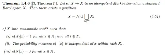
Recently, I stumbled across a new paper in categorical probability. Interestingly, they prove a result which may be formulated in purely measure-theoretic terms about which they note that
"As far as we know, this strengthening is new, and in particular no measure-theoretic proof exists to date."
This makes me wonder about whether one can prove this in a measure-theoretic way, without the tools from categorical probability they developed. The point of this post is to state the result and explain the definitions from a viewpoint of measure theory. My question then is:
Can we prove this Theorem with purely measure-theoretic tools, meaning without the tools of categorical probability used in the paper?
Main Theorem
Every idempotent Markov kernel between standard Borel spaces is balanced and splits.
For further context, this Theorem is a stronger version of the more well-known Theorem due to Blackwell, which the authors formulate as follows:
For a reference, see "Idempotent Markoff Chains" by Blackwell.
Definitions
Standard Borel Space:
We say that $(X,\Sigma)$ is a standard Borel space if $X$ is metrizable with metric $d$ such that $\Sigma$ is the Borel-$\sigma$-algebra generated by the topology of $(X,d)$ and $(X,d)$ is separable and complete.
Markov Kernel:
Let $(X,\mathcal A)$ and $(Y,\mathcal B)$ be measurable spaces. A Markov Kernel from $(X,\mathcal A)$ to $(Y,\mathcal B)$ is a map $\kappa:X\times\mathcal B\rightarrow [0,1]$ such that
- For every $B\in\mathcal B$ the map $x\mapsto \kappa(x,B)$ is $\mathcal A$-measurable.
- For every $x\in X$ the map $B\mapsto \kappa(x,B)$ is a probability measure on $(Y,\mathcal B)$.
Example: If we consider Markov Chains on a discrete space, say $S:=\{1,2\}$, usually described by a transition matrix $$e:=\begin{pmatrix}\frac{1}{4} & \frac{3}{4} \\ \frac{2}{5} & \frac{3}{5} \end{pmatrix}$$ then our spaces are $X=Y=S$ with their $\sigma$-algebras being the power set of $S$. The associated Markov Kernel $\kappa$ then is given by $$\begin{align*}\kappa(1,\{1\})&= \frac{1}{4}, \hspace{1cm}\kappa(1,\{2\})=\frac{3}{4} \\ \kappa(2,\{1\})&=\frac{2}{5}, \hspace{1cm}\kappa(2,\{2\})=\frac{3}{5}\end{align*}$$where one may interpret $\kappa(x,B)$ as $\mathbb P[X_1\in B|X_0=x]$ if $(X_n)_{n\in\mathbb N}$ is a Markov Chain with transition matrix $e$.
Composition of Markov Kernels
Let $(X,\mathcal A), (Y,\mathcal B), (Z,\mathcal C)$ be three measurable spaces and let $\kappa$ be a Markov Kernel from $X$ to $Y$, let $\lambda$ be a Markov Kernel from $Y$ to $Z$. We define the composition of the two kernels $\lambda\circ \kappa$ by $$(\lambda\circ \kappa)(x,dz):=\int_Y \lambda(y,dz)\kappa(x,dy)$$
Example: If we consider again the case of a discrete state space, we may represent Markov Kernels as stochastic matrices. Composition of two Kernels then equates to the product of the corresponding matrices.
We may now view Markov Kernels as morphisms.
Idempotence:
We say an morphism $e:X\rightarrow X$ is idempotent if it satisfies $e\circ e = e$.
Example: Examples of idempotent transition kernels on the state space $S:=\{1,2\}$ would be $$e_1=\begin{pmatrix}1 & 0 \\ 0 & 1\end{pmatrix},\hspace{1cm}e_2=\begin{pmatrix}\frac12 & \frac12 \\ \frac12 & \frac12\end{pmatrix}$$
Splitting:
Given an idempotent $e:X\rightarrow X$, we say that $e$ splits if there exists a $T$ and morphisms $$\iota:T\rightarrow X, \hspace{1cm} \pi:X\rightarrow T$$ such that $$\pi\circ \iota =\text{id}_T, \hspace{1cm} \iota\circ \pi=e$$
Example: (Example 4.1.4.)
Consider the discrete state space $S:=\{1,2\}$ and define a Markov Chain on $S$ by the transition kernel $$e=\begin{pmatrix}\frac12 & \frac12 \\ \frac12 & \frac12\end{pmatrix}$$ Then for $$\iota:=\begin{pmatrix}\frac12 \\ \frac12 \end{pmatrix}, \hspace{1cm} \pi:=\begin{pmatrix} 1 & 1\end{pmatrix}$$ we see that $\pi\circ\iota =\text{id}$ as well as $\iota\circ \pi=e$. (Here composition is considered as matrix-multiplication).
Balanced:
We say that $e$ is balanced if for every invariant distribution $\pi$ of $e$, meaning $e\pi=\pi$, we have that a Markov Chain with transition kernel $e$ and initial (stationary) distribution $\pi$ is reversible.
(I am not entirely sure that I understood this definition correctly. Please take a look at Definition 4.1.1 and Proposition 4.1.10 in the paper and correct me if you feel like I am stating the wrong definition here)
