Limiting Distribution with Successive Transformations

Question

I am not sure if this is a new problem but it is one that I thought up and have been working on for some time. Alas, I have been unable to develop a complete solution to the problem and would be interested if there are any useful techniques or insights that the community could provide.

I am looking for the continuous PDF $X$ that exists over $[0,1]$ and has the following relationship with is transformation:

\begin{equation} X \sim \frac{n}{n+X} \end{equation}

where $n \overset{iid}{\sim} U(0,1)$. What I am trying to convey here is that taking any number of transformations of the form $\frac{n_1}{n_1+X}$, $\frac{n_2}{n_2+X}$, etc. does not change the distribution $X$ for which we are looking. Furthermore, successive transformations such as $\frac{n_2}{n_2+\frac{n_1}{n_1+X}}$ and so on result in the same distribution $X$ for which we are looking.

Attempt 1

The first approach I took was took was to try to solve for $X$ by solving for the combination of random variates $n_1, n_2, ...$ and then performing the transformation on them. This became very messy and very quickly. Alas, this solution did not provide the limiting distribution but it did provide an insight.

Each successive addition of a random variate changed the distribution for $X$. Therefore, it did not seem that standard substitution techniques may be helpful with this type of problem.

Attempt 2

I noticed that the distribution on the interval from $[0,\frac{n}{n+1}]$ was always in the form of $\frac{c}{(X-1)^2}$, where $c$ is some constant. If this was the form of the limiting distribution for that interval, then perhaps I could apply the transformation on that segment of the distribution to gain insight about the remaining distribution $X$. This too became very messy, very quickly but with the help of Mathematica, I was able to get an approximation of the distribution which would seems much closer to the real distribution than in my first attempt. The results I obtained were (apologies for the math wall):

\begin{align} \frac{-X+(1-2 X) \log \left(\frac{X}{2 X-1}\right)+1}{2 (X-1)^2 (2 X-1)} && \frac{2}{3}\leq X<1 \\ \frac{1}{48} (-25) \left(6 \text{Li}_2(-3)-3 \left(\text{Li}_2\left(\frac{1}{4}\right)+6\right)+\pi ^2-6 \log ^2(2)+\log (3) \log (64)+\log (2985984)\right) && 5 X=3 \\ \frac{\text{Li}_2\left(\frac{1}{4}\right)+4+2 \log ^2(2)-3 \log (3)}{4 (X-1)^2} && 0<X\leq \frac{1}{2} \\ \frac{12 (2 X-1) \text{Li}_2\left(\frac{X-1}{2 X-1}\right)-48 X+\pi ^2 (2 X-1)+12 ((2 X-1) \log (1-X)-2 X) \log (X)+12 \left((1-2 X) \log \left(-\frac{(X-1) X}{2 X-1}\right) \log (2 X-1)+X \log ((3-2 X) X-1)\right)-24 \tanh ^{-1}(1-2 X)+36}{24 (X-1)^2 (2 X-1)} && \frac{3}{5}<X<\frac{2}{3} \\ \frac{\text{Li}_2\left(\frac{1}{4}\right) (2 X-1) (2-3 X)^2-2 (2-3 X)^2 (2 X-1) \text{Li}_2\left(\frac{X}{3 X-2}\right)+2 (2 X-1) (2-3 X)^2 \text{Li}_2\left(\frac{1-2 X}{2-3 X}\right)+33 X^2 \log \left(\frac{54}{X}-81\right)+2 \log \left(\frac{1}{X-1}+3\right) \left(21 X^2+\left(33 X^2+4\right) \log \left(\frac{X}{2 X-1}\right)\right)+2 \left(-9 X^3 \log \left(-27 (2-3 X)^2\right)+X \left(9 X^2 \log ((X-1) X)+2 \left(9 X^2+10\right) \log \left(\frac{2}{X}-3\right) \log (2 (X-1))+33 X \log \left(\frac{2 (X-1)}{3 X-2}\right) \log \left(\frac{X}{2-3 X}\right)+10 \log \left(\frac{X}{54-81 X}\right)\right)+\log (X-1) \left(-2 \left(9 X^2+10\right) X \log \left(\frac{2}{X}-3\right)-\left(33 X^2+4\right) \log \left(\frac{1-2 X}{3 X-2}\right)+16 X\right)+\left(\left(33 X^2+4\right) \log \left(\frac{1-2 X}{3 X-2}\right)-16 X\right) \log (3 X-2)\right)-\frac{1}{6} (2 X-1) (2-3 X)^2 \left(\pi ^2-12 \left(3+\log ^2(2)\right)\right)+\log \left(\frac{1}{(X-1)^8}\right)-4 \log (X)+8 \log \left(\frac{2 (X-1)}{3 X-2}\right) \log \left(\frac{X}{2-3 X}\right)+12 \log (6-9 X)}{4 (2 X-1) \left(3 X^2-5 X+2\right)^2} && \frac{1}{2}<X<\frac{3}{5} \\ 0 && X>1\lor X<0 \\ \text{Indeterminate} && \text{True} \\ \end{align}

Unfortunately, this approach does not seem to work well beyond the first two iterations and this is the best approximation I can get.

Observation

There may not be a feasible closed form solution to this problem. It seems as if the intervals for the individual sections may continue to break in accordance with fractions associated with the Fibonacci numbers: 1/2, 3/5, 8/11, etc. I haven't proven yet that this is indeed the case but if it is that way then a closed form solution is certainly not possible.

Additional Desire I am not sure if this is yet possible either but I am trying to track how the maximum value of the distribution progresses over time. Even if there is no closed form for this distribution I wonder if there is a way that you can find a closed form solution for the maximum value of for the values for $x=0,1$.

As always, I appreciate any insights from the math hive mind!

Answer 1

Existence of a density for $X$. Let $\mu$ denote the law of $X$ and suppose it solves the equation $$X\stackrel d=\frac U{U+X}=\left(1+\frac XU\right)^{\!-1}$$ where $U\sim\text{Uniform}(0,1)$ is independent of $X$. Then for every bounded measurable function $g$: \begin{align*} \Bbb E[g(X)]&=\int\int_0^1g\!\left(\left(1+\frac xu\right)^{-1}\right)\,\mathrm du\,\mu(\mathrm dx)\\[.4em] &=\iint x\,\mathbf1_{\left\{0<v(1+x)<1\right\}}\frac{g(v)}{(1-v)^2}\,\mathrm dv\,\mu(\mathrm dx)\\[.4em] &=\int_0^1\mathrm g(v)\left(\frac 1{(1-v)^2}\int_0^{\Phi(v)}x\,\mu(\mathrm dx)\right)\,\mathrm dv \end{align*} with $\Phi(v):=1\wedge(\frac1v-1)$, where we applied the change of variable $$\left\{\begin{aligned} v&=\left(1+\frac xu\right)^{-1},\\[.6em] \mathrm dv&=\frac{(1-v)^2}{x}\,\mathrm du, \end{aligned}\right.$$ and Fubini's theorem. This shows that $X$ admits a Lebesgue density on $(0,1)$, $\mu(\mathrm dx)=f(x)\,\mathrm dx$, such that, for every $v\in(0,1)$, $$f(v)=\frac 1{(1-v)^2}\int_0^{\Phi(v)}xf(x)\,\mathrm dx.\tag{$\star$}$$

---

Expression of the density. Let $\phi>0$ be the unique solution to $v=\Phi(v)$, i.e., $\phi=\frac{\sqrt5-1}2\approx0.618\ldots$ Write $(0,1)=I_1\cup I_2\cup I_3\cup I_4$, with $$I_1:=\left(0,\frac12\right],\quad I_2:=\left(\frac12,\phi\right],\quad I_3:=\left[\phi,\frac23\right),\quad I_4:=\left[\frac23,1\right)\!.$$ Let $f_j(v):=f(v)$ for $v\in I_j$ and let us determine $f$ on each sub-interval $I_j$, $j\in\{1,2,3,4\}$.

First, let $m:=\Bbb E[X]=\int_0^1xf(x)\,\mathrm dx$. Since $\Phi(I_1)=\{1\}$, Eq. $(\star)$ gives $$f_1(v)=\frac m{(1-v)^2}.$$ Now for $v\in I_4$, $(0,\Phi(v)]\subseteq I_1$, so Eq. $(\star)$ gives \begin{align*}f_4(v)&=\frac m{(1-v)^2}\int_0^{\Phi(v)}\frac x{(1-x)^2}\,\mathrm dx\\[.4em] &=\left(\frac1{(1-v)(1-2v)}+\frac{\log\!\left(2-\frac1v\right)}{1-v^2}\right)m.\end{align*}

It remains to compute $f_2$ and $f_3$. Since $\Phi(I_3)=I_2$ and $(0,\Phi(\frac23)]=I_1$, $(\star)$ translates into \begin{align*} f_3(v)&=\frac1{(1-v)^2}\left(\int_{I_1}xf_1(x)\,\mathrm dx+\int_{\frac12}^{\frac1v-1}xf_2(x)\,\mathrm dx\right)\!\\[.4em] &=\frac1{(1-v)^2}\left(\frac{f_4\!\left(\frac23\right)}9 +\int_{\frac12}^{\frac1v-1}xf_2(x)\,\mathrm dx\right)\!.\tag{$1$} \end{align*} Similarly, for $v\in I_2$, we have $\Phi(v)\in I_3\iff v\in(\frac35,\phi]$ and $\Phi(v)\in I_4\iff v\in(\frac12,\frac35]$. Thus, for $v\in(\frac35,\phi]$, \begin{align*} f_2(v)&=\frac1{(1-v)^2}\left(\int_{I_1}xf_1(x)\,\mathrm dx+\int_{I_2}xf_2(x)\,\mathrm dx+\int_\phi^{\frac1v-1}f_3(x)\,\mathrm dx\right)\\ &=\frac1{(1-v)^2}\left(\phi^4f_3(\phi)+\int_\phi^{\frac1v-1}f_3(x)\,\mathrm dx\right)\!,\tag{$2$} \end{align*} and, for $v\in(\frac12,\frac35]$, \begin{align*} f_2(v)&=\frac1{(1-v)^2}\left(\int_{I_1}xf_1(x)\,\mathrm dx+\int_{I_2}xf_2(x)\,\mathrm dx+\int_{I_3}xf_3(x)\,\mathrm dx +\int_{\frac23}^{\frac1v-1}xf_4(x)\,\mathrm dx\right)\\[.4em] &=\frac1{(1-v)^2}\left(\frac4{25}f_2\!\left(\frac35\right)+\int_{\frac23}^{\frac1v-1}xf_4(x)\,\mathrm dx\right)\!.\tag{$2'$} \end{align*} One may plug the expression of $f_4$ into $(2')$, then go back to $(1)$ to get $f_3$, and then completely get $f_2$ using $(2)$. It becomes indeed quite messy, though (Mathematica was only able to express the involved integrals using polylog functions).

Answer 2

Not a full answer, rather a sketch:

We want to find a random variable $X$ over $[0,1]$ such that $Z =\frac{Y}{Y+X}$ has the same distribution as $X$, where $Y$ is uniform over $[0,1]$ and independent of $X$. Let's assume that such density $f_X= f_Z$ exists.

Now for any $0<a<1$:

$$P(Z\le a) = P(Y \le (Y+X)a) = P(Y \le b X)$$

where $b(a)=\frac{a}{1-a}$.

In the range $0<a<\frac12 \iff 0<b<1 $ we have

$$P(Z\le a) = \int_0^1 f_X(x) P(Y \le bx) dx= \int_0^1 f_X(x)\, b\, x \, dx= \frac{a}{1-a} \, \mu \tag 1$$

This implies that $Z$, (and, hence $X$) in that range has a density of the form $$f_X(x)=\frac{\mu}{(1-x)^2} \hskip{1cm} 0 < x < \frac12 \tag 2$$

Next we consider the range $\frac12<a< \frac23 \iff 1<b< 2$

This gives a new condition that should allow us to get $f_X(x)$ in the range $[\frac23,1]$ based on the already computed values over $[0,\frac12]$. Things seem to get somewhat messy, though...

Update:

Here's the expression I found for $2/3<x<1$:

$$f_X(x) = \frac{\mu}{{\left( 1-x\right) }^{2}} \left( \frac{1-x}{2x-1}+ \log{\left( \frac{ 2x-1 }{x}\right) }\right) \tag 3$$

And, in general, the following equation applies:

$$ f_X(x) = \frac{1}{(1-x)^2}\int_0^{(1-x)/x} f_X(r) \, r \, dr \tag 4$$

with the restrictions $f_X(x) \ge 0 $ inside $[0,1]$, $f_X(x) = 0 $ outside, and $\int_0^1 f_X(x) dx=1$.

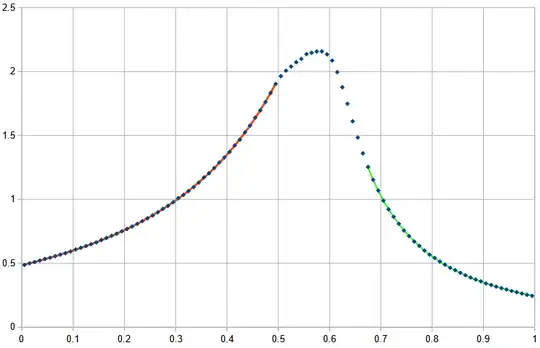
Simulations suggest there is indeed a stable density:

Dots correspond to my simulation. In red and green lines, the results from eqs $(2)$ and $(3)$

The empirical mean is $\mu=0.485985$