There are two things necessary to increase the definition of the image:
- Compute the modular form to higher accuracy, and
- Plot the modular form in a finer mesh.
In sage, the way to do the latter is with the plot_points parameter in complex_plot. By default, sage will evaluate the function on a $100 \times 100$ grid and interpolate between the points. This gives a pretty low-definition picture.
Let's include runnable code. Although I separate the code into chunks, think of all the code as a single code file, in that later code snippets depend on earlier code snippets.
The following code redoes what you've done. It computes a degree $39$ polynomial using the first 40 coefficients of $f$, the unique modular form (actually an Eisenstein series) of weight $4$ on $\mathrm{SL}(2, \mathbb{Z})$. Then it plots it.
# sage code
Htoq = lambda x: exp(2 * CDF.pi() * CDF.0 * x)
DtoH = lambda x: (-CDF.0 * x + 1) / (x - CDF.0)
Dtoq = lambda x: Htoq(DtoH(CDF(x)))
C.<t> = CC[]
M4 = ModularForms(1, 4)
f = M4.basis()[0]
coeffs = f.coefficients(list(range(40)))  # take 40 coefficients
fpoly = C(coeffs)  # interpret coeffs in the polynomial ring C.<t>
P = complex_plot(
  lambda z: fpoly(Htoq(z)),
  (-1, 1), (0.01, 2),
  aspect_ratio=1, figsize=[4, 4])
P.axes(show=False)
P
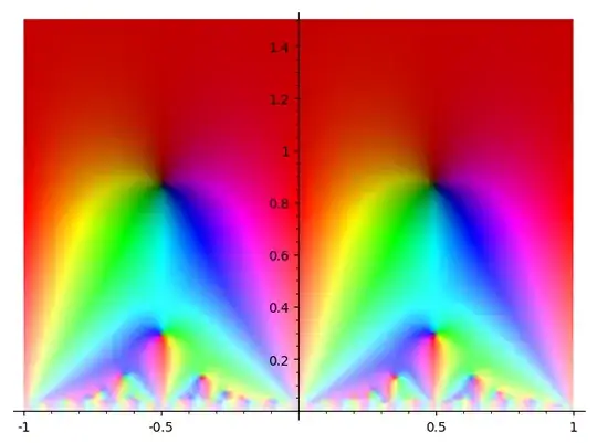
This makes the following image, from $40$ coefficients evaluated on a $100 \times 100$ grid.
We can instead evaluate it on a $500 \times 500$ grid with the following code change.
# continuing from above code
P = complex_plot(
  lambda z: fpoly(Htoq(z)),
  (-1, 1), (0.01, 2),
  aspect_ratio=1, figsize=[4, 4],
  plot_points=500   # <--- new line
)
P.axes(show=False)
P

Notice the higher resolution. The bands of color at the bottom are numerical artifacts from low precision evaluation of the modular form.
Using more coefficients is one way to increase the accuracy near the boundary. See the following code.
coeffs = f.coefficients(list(range(100)))  # <-- 100 coefficients
fpoly = C(coeffs)
P = complex_plot(
  lambda z: fpoly(Htoq(z)),
  (-1, 1), (0.01, 2),
  aspect_ratio=1, figsize=[4, 4],
  plot_points=500)
P.axes(show=False)
P
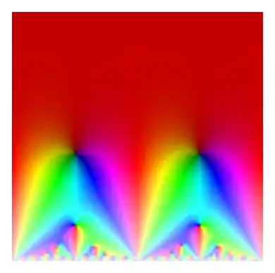
This gives the following picture.

Now there is almost no banding at the boundary. Similar techniques would work for other visualizations, such as on the Poincare disk.
P = complex_plot(
  lambda z: +Infinity if abs(z) >= 0.99
            else fpoly(Dtoq(z)) * exp(1.2 * CDF.pi() * CDF.0),
  (-1, 1), (-1, 1), aspect_ratio=1, figsize=[4,4],
  plot_points=500)
P.axes(show=False)
P
This gives the following image on the disk.
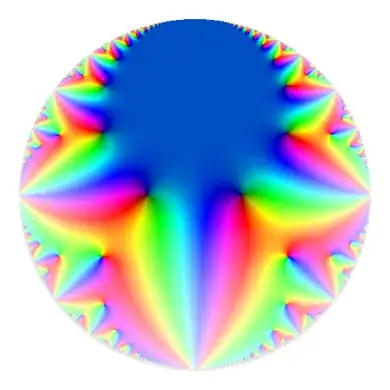
There is some banding around parts of the boundary from approximation problems.
I note that the argument factor exp(1.2 * pi * i) is there just to make the phase corresponding to real values blue, which is more pleasant than the default red. For the older images corresponding to modular forms in the LMFDB, we did the same thing more or less. (We now produce images like on this page, which use a different colormap. Reasons and methods for this are noted in this paper).
I'll also note that there are other ways to compute the modular form to higher accuracy. For level $1$, you can pullback each point to the fundamental domain (where the imaginary part is large, and thus the $q$-expansion converges rapidly). It is necessary to track the matrices used and use the modularity $f(\gamma z) = (cz + d)^k f(z)$.
I'll give sample code that does this, but with a small caveat: I use this code outside of sage in ways that allow this to be done faster or in different visualizations. I put code modified from what was used to make this video. It would be possible to do this a bit more simply using sage's concept of matrices, matrix multplication, and actions.
# sage code
Htoq = lambda x: exp(2 * CDF.pi() * CDF.0 * x)
DtoH = lambda x: (-CDF.0 * x + 1) / (x - CDF.0)
Dtoq = lambda x: Htoq(DtoH(CDF(x)))
C.<t> = CC[]
M4 = ModularForms(1, 4)
f = M4.basis()[0]
coeffs = f.coefficients(list(range(40)))  # only 40 coefficients
fpoly = C(coeffs)
def in_fund_domain(z):
    x = z.real()
    y = z.imag()
    if x < -0.51 or x > 0.51:
        return False
    if xx + yy < 0.99:
        return False
    return True
def act(gamma, z):
    a, b, c, d = gamma
    return (az + b) / (cz + d)
def mult_matrices(mat1, mat2):
    a, b, c, d = mat1
    A, B, C, D = mat2
    return [aA + bC, aB + bD, cA + dC, cB + dD]
Id = [1, 0, 0, 1]
def pullback(z):
    """
    Returns gamma, w such that gamma(z) = w and w is
    (essentially) in the fundamental domain.
    """
    z = CDF(z)
    gamma = Id
    count = 1
    while not in_fund_domain(z):
        if (count > 1000): print(z, count)
        count += 1
        x, y = z.real(), z.imag()
        xshift = -floor(x + 0.5)
        shiftmatrix = [1, xshift, 0, 1]
        gamma = mult_matrices(shiftmatrix, gamma)
        z = act(shiftmatrix, z)
        if xx + yy < 0.99:
            z = -1/z
            gamma = mult_matrices([0, -1, 1, 0], gamma)
    return gamma, z
def smart_compute(z):
    gamma, z = pullback(DtoH(z))
    a, b, c, d = gamma
    return (-cz + a)4  fpoly(Htoq(z))
P = complex_plot(
  lambda z: +Infinity if abs(z) >= 0.99
            else smart_compute(z) * exp(1.2 * CDF.pi() * CDF.0),
  (-1, 1), (-1, 1), aspect_ratio=1, figsize=[6, 6],
  plot_points=500)
P.axes(show=False)
P
Using only 40 coefficients, this gets a very high fidelity image (but takes approximately 20 seconds to run on my machine).

For higher level, it is not possible to always choose points in the fundamental domain with large imaginary part. Alternative methods are available, but they're frequently rather annoying in my experience.