There is none, even if $f$ is allowed to be a distribution and if the convolution is understood as a convolution of distributions.
I interpret the question as allowing $f$ to be defined on $\mathbb{R}$ with null value outside of $]0,1[$.
I - No solutions in the space of tempered distributions
Fourier transforms of the right hand side (RHS) can be considered, if you allow Cauchy principal values (denoted by a P before the integration symbol). Then its Fourier transform is:
$$ P\int_{-\infty }^{\infty } \frac{e^{-i \text{sx}}}{1-x} \, dx = i \pi e^{-i s} \text{sgn}(s)$$
On the left hand side, the weakest hypothesis on $f$ compatible with a Fourier transform analysis of the question is that the functional $T_f$ defined in the space of Schwartz functions by $ T_f(\phi)= \langle f, \phi \rangle$ be a tempered distribution. This is the assumption that is made for what follows to make sense. It is later shown that this assumption cannot hold true.
It is a classical result that the Fourier transform of $T_f$ exists (see [3]). For simplicity, in what follows, the functional notation will be dropped, so $f*f$ should for example be interpreted as $T_{f}*T_{f}$ or $(T_{f}*T_{f})(\phi)$ depending on context. I interpret the question as implicitly positing the assumption that $f*f$ exists in the sense of distributions (which is for example the case if $f$ is locally integrable, a much weaker condition than $f \in \mathbb{L^1(R)}$).
Let us denote by $F$ the Fourier transform of $f$ under these assumptions.
The convolution theorem for Fourier transforms remains valid (see [4]).
We now have:
$$ {F[s]}^2 = i \space \pi \space e^{-i s} \text{sgn}(s)$$
(See 1, table number 309, or 2 page 64 for the sine transform).
Considering that the square root is a multi-valued complex function, the banches of the square root will be indexed by integer $k$ to obtain the Fourier transform:
$$ F[s] = \sqrt\pi e^{i (-s/2 + \space \text{sgn}(s) \pi/4 + \space k \pi) }$$
each branch of which is continuous on $\mathbb{R}^*$. It is obviously invertible and computing the inverse Fourier transform yields:
$$ f_0(x) = \epsilon \space \frac{\sqrt{\frac{2}{\pi}}}{1 - 2 x} \text{, with} \space \epsilon² = 1. $$
There is a pole at $\frac{1}{2}$, so either your convolution tolerates Cauchy principal values or not, in which latter case the negative result is straightforward. Granting the option of a Cauchy principal value convolution, $f_0$ is now integrable in the Riemann sense and one can easily check that its integral over $[0, 1]$ is zero.
It is obvious that $f_0$ cannot be null outside of $[0, 1]$, and as $f_0 = f$ if the question admits a solution in the space of tempered distributions, it follows that the question admits no solution in this space.
Even if the value of $f_0$ outside of $[0, 1]$ were by some extra assumption finally not considered at all, the direct computation of the (principal-valued) convolution itself is not possible for $ x \ge \frac{1}{2}$, and for $x < \frac{1}{2}$, it yields:
$$ (f_0*f_0)(x) = \frac{\ln (1-2 x)}{\pi (x-1)}$$
which is equal to the RHS only at one point of the interval ($x = \frac{1}{2} \left(1-e^{-\pi }\right)$).
II - No solutions in the space of distributions with support contained in $\mathbb{R^+}$ that have a Laplace transform
We now remove the requirement for a tempered distribution and replace it by the other requirement that:
$$\text{The space of distributions has left-bounded support included in} \, \, \mathbb{R^+} \, (R_1).$$
We add the requirement that:
$$e^{-\xi} T_{f} \text{ be a tempered distribution for all } \xi > \xi_0 \, \, (R_2).$$
This is a less stringent condition than the one used in I.
Now, the Laplace transform of $f$ at $p$, which will simply be denoted by $L(p)$, exists for $p > \xi_0$, for some given $\xi_0 > 0$.
The convolution $f*f$ now exists without further assumptions to be made. Notice that, $\theta$ being the Heaviside step function:
$$ \int_{0}^{1} f(u) f(x-u) \, du = \int_{0}^{1} \theta(x-u) \, f(u) f(x-u) \, du$$
as, if $u > x$, then $f(x-u) = 0$ by hypothesis.
So that:
$$ \int_{0}^{1} f(u) f(x-u) \, du = \int_{0}^{x} f(u) f(x-u) \, du$$
It is known that the Laplace transform $L(p)$ of $f*f$, in the sense of the convolution of distributions, is $L(p)^2$ (see [5]). It is equal to the Laplace transform of the left-hand side, owing to the above equation.
On the other hand, the Laplace transform of the RHS, granting Cauchy principal value integration, can be shown to be:
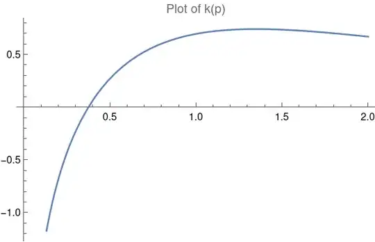
$$k(p) = E_i(p) e^{-p}$$
for $p > 0$ arbitrary.
Now, it suffices to notice that, for $p < 0.3$, the above value is negative, which is a contradiction.
It follows that there is no solution to the problem in the space of distributions satisfying the (relatively weak) requirements $(R_1)-(R_2).$
III- Final part of the demonstration
As the interval of integration is included in $\mathbb{R^+}$ and $f$ vanishes elsewhere, the support of $f$ necessarily satisfies $(R_1)$, so $(II) \Rightarrow (I).$ This would not be true if, for example, the lower bound of integration were $-1$.
Finally, all the conditions of (I) and (II) will be satisfied if $T_f$ has compact support, as a distribution with compact support is necessaritly tempered (see [6]).
Let us show now that a solution $T_f$, if it exists, must have compact support, which will prove the negative answer to the question.
First, if $T_f$ vanishes almost everywhere within $]0, 1[$, then each non-zero of $T_f$ in the interval is an adherent point of a sequence of zeros, hence the support of the distribution is a null set (of zero measure) and the integrals vanish. It is obvious that there can be no solution to the problem in this case.
As a consequence, the support of the distribution must contain a open subset $A \subset ]0,1[$ of non-zero measure. Let us consider the union $\Omega$ of such open subsets. It still is an open subset of non-zero measure and it contains all the interior of the support. In other words, $T_f$ vanishes only outside of $\Omega$ with $\, \mu(\Omega) > 0$.
In this case, by the Borel-Lebesgue theorem, the closure $\bar \Omega$ of $\Omega$, which is the support of $T_f$, will be compact and of non-zero measure too. This completes the demonstration.
1 https://en.wikipedia.org/wiki/Fourier_transform
2 Erdélyi, Arthur, ed. (1954), Tables of Integral Transforms, vol. 1, McGraw-Hill.
[3] van Dijk, G. (2013), Distribution Theory: Convolution, Fourier Transform, and Laplace Transform, De Gruyter, 7.8 p. 64.
[4] Ibid. 7.8 p. 65.
[5] Ibid. 8.3 p.76.
[6] Ibid. 7.6 p.60.
