Least Squares fit to closest convex function

Question

I encountered a task where I have some discrete set of data points $(x_1, y_1), \ldots, (x_n, y_n)$, where $x_1 < x_2 < \ldots < x_n$.
The discrete function graph they form should ideally be convex, but due to some noise and errors it deviates slightly from being convex everywhere.
I would therefore like to replace the $\{ y_i \}_{i=1, \ldots, n}$ with values $\{ w_i \}_{i=1, \ldots, n}$ so that the new function graph given by the points $(x_1, w_1), \ldots, (x_n, w_n)$ is convex and the squared difference $$ \sum_{i=1}^n (y_i - w_i)^2 $$ is minimal.

I don't want to assign any parametric model for the $\{ w_i \}_{i=1, \ldots, n}$ unless I have to, since it should not be necessary to do so. This problem should be solvable anyway.

Maybe this is some well known stuff. I would then be thankful if anyone could point me to some good references.
One can of course write it as a general optimization problem in the $n$ unknown variables $\{ w_i \}_{i=1, \ldots, n}$ with a lot of inequalities as side conditions representing the convexity condition.
However, I would prefer some simpler solution, if it exists, or some algorithm that does not give the perfect optimal result, but still a convex graph that approximates the old graph "good enough".

"with a lot of inequalities as side conditions representing the convexity condition": you only need one inequality per data point (forcing it to be below the line connecting its neighbors) — LinAlg, Feb 05 '21 at 16:04
Yes, that is what I mean, one inequality per interior data point, which becomes quite a lot if you have many points. — Jesper Tidblom, Feb 06 '21 at 08:13
How many is 'many'? The Hessian of the Lagrangian has very sparse and banded structure. I would be surprised if problems with a million points pose a problem for the interior point algorithms in gurobi/cplex/mosek. — LinAlg, Feb 06 '21 at 14:28
Sure, I don't have access to those premade functions/algorithms at my work though. And I would prefer not to reimplement those optimizers at the moment at least, since that would be quite time consuming. — Jesper Tidblom, Feb 08 '21 at 06:39
I do not understand based on what the $w_i$ must be chosen. It says that the $(x_i,w_i)$ should form a convex graph, but what relation do they have with the $y_i$? — Isidor Konrad Maier, Nov 05 '24 at 10:33

Cesareo · Accepted Answer · 2021-02-08T10:15:59.017

Using a cubic spline we can easily obtain good convex/concave fitting.

Follows a MATHEMATICA script which smooths the data imposing convexity/concavity as required. The quadratic spline has n equal spaced intervals, from 0 until tmax, with coefficients at each interval given by a[k], b[k], c[k] or as $s(k,t) = a_k + b_k(t-k\delta)+c_k(t-k\delta)^2$

Unprotect["`*"]; 
ClearAll["`*"];
fl[a_, b_, c_, delta_, t_, n_] := Sum[(UnitStep[t - k delta] - UnitStep[t - (k + 1) delta]) (a[k] + b[k] (t - k delta) + c[k] (t - k delta)^2), {k, 0, n}]
n = 10;
tmax = 2;
delta = tmax/n;
kappa = -0.3;
fl0 = fl[a, b, c, delta, t, n];

After the spline formal definition the continuity conditions are introduced.

For[k = n - 1, k >= 0, k--,
  fl0 = fl0 /. {a[k + 1] -> a[k] + delta b[k] + delta^2 c[k] , 
                b[k + 1] -> b[k] + 2 delta c[k]}
]

so the final independent parameters are given in

vars = Join[{a[0], b[0]}, Table[c[k], {k, 0, n}]];

Now we define a function with concave epigraph, generating data added to noise

y[x_] := x (2 - x) + x/2
data = Table[{x, y[x] + RandomReal[{-0.1, 0.1}]}, {x, 0, tmax, 0.1}]
gr1 = ListPlot[data, PlotStyle -> {Thick, Red}];

Follows a minimization procedure to determine de spline coefficients.

obj = Sum[Abs[(fl0 /. {t -> data[[k, 1]]}) - data[[k, 2]]], {k, 1, 
Length[data]}];

Due to epigraph concavity the condition is $c_k < \kappa$. Here $\kappa$ is the minimum acceptable to avoid the inclusion of line segments $(c_k = 0)$.

restr = Table[c[k] < kappa, {k, 0, n}];(* concave epigraph *)

Now the minimization results: result1 with imposed concavity and result2 without conditions.

sol1 = NMinimize[Join[{obj, restr}], vars]
sol2 = NMinimize[obj, vars]

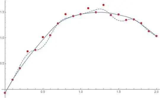
Follows a graph shoving in red the data points, in dashed blue the unrestricted minimization and in blue continuous the conditioned minimization.

fl01 = fl0 /. sol1[[2]];
gr21 = Plot[fl01, {t, 0, tmax}];
fl02 = fl0 /. sol2[[2]];
gr22 = Plot[fl02, {t, 0, 2}, PlotStyle -> Dashed];
Show[gr1, gr21, gr22, PlotRange -> All]

NOTE

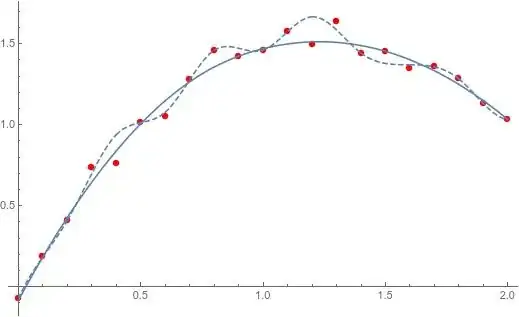
The same data processed with a cubic spline. In this case the concavity/convexity is respectively $d_k > 0, \ \ d_k < 0$

Least Squares fit to closest convex function

1 Answers1

Linked