Why do we define $\lambda = np$ when deriving the Poisson distribution from the Binomial distribution? How do you come up with this definition? I couldn't find a good intuitive explanation of why this is done. My textbook and professors just stated this definition and then made a derivation.
-
2The parameter $\lambda$ specifies the mean number of events for a Poisson distribution. The mean of a Binomial distribution is $np$, so it would make sense for the two quantities to match. – JKL Jan 21 '21 at 04:29
-
Does this answer your question? What is the intuition behind the Poisson distribution's function? – Akalanka Jan 21 '21 at 04:30
1 Answers
You are not 'deriving' the Poisson distribution from the binomial distribution. In some circumstances (especially when binomial $p$ is small and binomial $n$ is large) it is possible to find a Poisson distribution that approximates the a binomial distribution. Such an approximation works best if the Poisson mean $\lambda$ matches the binomial mean $np.$
Here is a table, made using R, comparing selected probabilities for $\mathsf{Binom}(n = 200, p = 0.1)$ and $\mathsf{Pois}(\lambda = 20).$
(You can ignore line numbers in [ ]s.)
k = 5:35
b.pdf = round(dbinom(k, 200, .1), 4)
p.pdf = round(dpois(k, 20), 4)
abs.dif = abs(b.pdf - p.pdf)
cbind(k, b.pdf, p.pdf, abs.dif)
Table:
       k  b.pdf  p.pdf abs.dif
 [1,]  5 0.0000 0.0001  0.0001
 [2,]  6 0.0001 0.0002  0.0001
 [3,]  7 0.0003 0.0005  0.0002
 [4,]  8 0.0009 0.0013  0.0004
 [5,]  9 0.0021 0.0029  0.0008
 [6,] 10 0.0045 0.0058  0.0013
 [7,] 11 0.0087 0.0106  0.0019
 [8,] 12 0.0153 0.0176  0.0023
 [9,] 13 0.0245 0.0271  0.0026
[10,] 14 0.0364 0.0387  0.0023
[11,] 15 0.0501 0.0516  0.0015
[12,] 16 0.0644 0.0646  0.0002
[13,] 17 0.0775 0.0760  0.0015
[14,] 18 0.0875 0.0844  0.0031
[15,] 19 0.0931 0.0888  0.0043
[16,] 20 0.0936 0.0888  0.0048
[17,] 21 0.0892 0.0846  0.0046
[18,] 22 0.0806 0.0769  0.0037
[19,] 23 0.0693 0.0669  0.0024
[20,] 24 0.0568 0.0557  0.0011
[21,] 25 0.0444 0.0446  0.0002
[22,] 26 0.0332 0.0343  0.0011
[23,] 27 0.0238 0.0254  0.0016
[24,] 28 0.0163 0.0181  0.0018
[25,] 29 0.0108 0.0125  0.0017
[26,] 30 0.0068 0.0083  0.0015
[27,] 31 0.0042 0.0054  0.0012
[28,] 32 0.0024 0.0034  0.0010
[29,] 33 0.0014 0.0020  0.0006
[30,] 34 0.0008 0.0012  0.0004
[31,] 35 0.0004 0.0007  0.0003
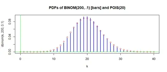
In the following graphical comparison, differences in probabilities less than 0.003 are difficult to distinguish.
hdr="PDFs of BINOM(200, .1) [bars] and POIS(20)"
k  = 0:40
plot(k, dbinom(k,200,.1), type="h", lwd=2,
      col="blue", main=hdr)
 points(k, dpois(k, 20), col="red")
 abline(h = 0, col="green2")
 abline(v = 0, col="green2")
Note: Binomial probabilities $X\sim\mathsf{Binom}(n,p)$ have $P(X > n) = 0.$ Technically, Poisson probabilities never reach $0,$ no matter how far into the right tail you go. But for practical purposes the probabilities become too small to be of importance beyond some finite point. In particular, for $Y \sim\mathsf{Pois}(\lambda= 20),$ we have $P(Y > 40) \approx 0.$ Markov's inequality does not give 'tight' bound, but does guarantee $P(Y \ge k\lambda) \le \lambda/k\lambda = 1/k.$
1 - ppois(40,20)
[1] 2.542632e-05
- 52,418
-
1At the end there you mean $P(X>n)=0$. Also, the decay of the Poisson in the tail is much faster than you get from Markov's inequality. – Ian Jan 23 '21 at 00:18
-
@ Ian: Fixed typo; thanks. // The Markov inequality is admittedly a poor bound--just making the point decay is eventually headed to $0,$ Chebyshev's inequality does better. If $\lambda$ is large enough for Poisson to be approximately normal, then there's little probability beyond $5\lambda.$ // Trying to keep discussion at very elementary level of question. – BruceET Jan 23 '21 at 00:39
-
So you're saying that the first time someone approximated the Binomial with Poisson, the Poisson distribution was already known? That is, the Poisson distribution wasn't discovered as a consequence of taking $n$ and $p$ to their limits in the Binomial? I guess I was confused because I thought this is how you derive the Poisson distribution. – jlcv Jan 23 '21 at 20:54
-
Supp0se you have a deck of 2000 cards of which 200 are red and the rest black. You are going to draw five cards and wonder your chances of getting no red cards. If you say that you'll get 1/10 reds per draw on avg, then you can say the ans is $P(X=0)=e^{-.5} = 0.6065307,$ where $X\sim POIS(.5),$ ignoring that there are finitely many cards. You can do samp w/ repl. to get $P(X=0) = .9^5 = 0.59049,$ where $X \sim BINOM(0, 5, .1).$ Or you can sample w/out repl and get the hypergeometric prob $P(X=0) = 0.5901615.$ All 3 approaches lead to probabiliy about $0.59.$ Or you can prove limit theorems. – BruceET Jan 24 '21 at 00:09
