26

It’s well known that the geometric mean of a set of positive numbers is less sensitive to outliers than the arithmetic mean. It’s easy to see this by example, but is there a deeper theoretical reason for this?

How would I go about “proving” that this is true? Would it make sense to compare the variances of the GM and AM of a sequence of random variables?

StubbornAtom
  • 17,932

2 Answers2

75

The geometric mean is the exponential of the arithmetic mean of a log-transformed sample. In particular,

$$\log\left( \biggl(\prod_{i=1}^n x_i\biggr)^{\!1/n}\right) = \frac{1}{n} \sum_{i=1}^n \log x_i,$$ for $x_1, \ldots, x_n > 0$.

So this should provide some intuition as to why the geometric mean is insensitive to right outliers, because the logarithm is a very slowly increasing function for $x > 1$.

But what about when $0 < x < 1$? Doesn't the steepness of the logarithm in this interval suggest that the geometric mean is sensitive to very small positive values--i.e., left outliers? Indeed this is true.

If your sample is $(0.001, 5, 10, 15),$ then your geometric mean is $0.930605$ and your arithmetic mean is $7.50025$. But if you replace $0.001$ with $0.000001$, this barely changes the arithmetic mean, but your geometric mean becomes $0.165488$. So the notion that the geometric mean is insensitive to outliers is not entirely precise.
heropup
  • 143,828
  • 2
    +1 Very nice explanation. But if the GM is the exponential of something, shouldn't that intuitively suggest that it should be sensitive to right outliers, since exponentials are very sensitive to errors to the right? – Ovi Apr 05 '20 at 03:32
  • 5
    @Ovi Consider a simple numerical example. $$\exp((\log 10 + \log 1000)/2) = 100,$$ and $$\exp((\log 10 + \log 2000)/2) = 141,$$ yet the arithmetic mean is nearly doubled. The reason is because the logarithm of right outliers takes place before the averaging, thus flattening out their contribution to the mean. Exponentiation of the final result only transforms the values back to the original scale. This is why I say "provide some intuition." It is not a formal proof, but an invitation to develop deeper understanding. – heropup Apr 05 '20 at 03:55
  • Ah I understand it better, thanks! – Ovi Apr 05 '20 at 04:03
  • @heropup Thank you for your fantastic answer. If possible, might you be able to recommend some books I can work through to be better equipped to reason through these kinds of problems myself? Should I learn more probability and statistics? Or numerical methods? – TheProofIsTrivium Apr 05 '20 at 05:58
  • 3
    Great answer. Tl;dr: the arithmetic mean is sensitive to additive outliers (ones whose distance from the rest of the data is large in magnitude); the geometric mean is sensitive to multiplicative outliers (ones whose logged ratio with the rest of the data is large in magnitude). – BallpointBen Apr 05 '20 at 19:23
6

We can even generalized this idea further - consider the definition of a power mean: $$\mu_p=\left(\frac{1}{n} \sum_{i=1}^n x_i^p \right)^\frac{1}{p}$$ We get the arithmetic mean when we plug $p=1$ and geometric mean when $p\rightarrow0$. It turns out that the lesser the value of $p$ the less impact the big numbers make and more impact small numbers make. Notice that for example even if $x_1$ is very close to zero the arithmetic mean will always be at least $\frac{x_2+x_3+\dots+x_n}{n}$ so it won't go down to zero. This is not the case for the other extreme - the arithmetic mean can be arbitrarily large only because of a single element. The same is true for all power means with $p>0$. For negative $p$ we have the reverse behaviour. Consider a harmonic mean (which is a reciprocal of an arithmetic mean of reciprocals and also a power mean with $p=-1$): $$\frac{n}{\sum_{i=1}^{n}\frac{1}{x_i}}$$ We see that even if $x_1$ is huge, it's reciprocal will still be bigger than zero making the whole mean less than: $$\frac{n}{\sum_{i=2}^{n}\frac{1}{x_i}}$$ But if only one element is very close to zero, it's reciprocal will be very big which will make the whole denominator large and thus make the harmonic mean go down to zero. Geometric mean, since it is a power mean with $p=0$ exhibits both these behaviours - it can grow big or small under the influence of just a single element. It seems bad ad first but one has to remember that it will be less sensitive to big outliers than any power mean with $p>0$ (like for example arithmetic mean) and less sensitive to small outliers than any power mean with $p<0$ (such as the harmonic mean) - so in some sense it can be a good compromise.

There are also two important special/border cases of the power mean, mainly $p \rightarrow \infty$ and $p \rightarrow -\infty$. In the first case, we just get the maximum and in the second minimum of the data. Obviously, as they are extremes, the maximum is completely sensitive to big outliers and completely insensitive to small ones whereas the minimum exhibits opposite behaviour. They are obviously a horrible example of a "mean" but can serve as a help in understanding general behaviour.

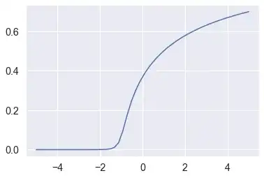
I've generated a random sample of million uniformly distributed numbers and computed their power means for different values of $p$. For $p=1$ we observe the mean of around $\frac{1}{2}$ which is a true mean of the distribution. For bigger values of $p$ we obtain bigger means, as always, but as you can see for $p<1$ we observe very small values of the mean. Also for bigger $p$ the mean seems to not be representative. So one has to make a choice depending on the distribution.

                                             Sensitivity to p

PROOF THAT GEOMETRIC MEAN IS A POWER MEAN FOR $p=0$:
We have thanks to the L'Hôpital's rule: $$\log u_0=\lim_{p\rightarrow 0}\frac{\log(\sum_{i=1}^n x_i^p)-\log(n)}{p}=\lim_{p\rightarrow 0}\frac{\sum_{i=1}^n x_i^p \log x_i}{\sum_{i=1}^n x_i^p}=\frac{1}{n}\sum_{i=1}^n \log x_i$$ So indeed: $$\mu_0=\exp\left(\frac{1}{n}\sum_{i=1}^n \log x_i \right)=\left(\prod_{i=1}^nx_i \right)^\frac{1}{n}$$

Bartek
  • 2,575