How do I apply regression techniques to data I think fits a differential equation?

Question

I have a calculus background and am beginning to learn about regression and statistical inference.

Let's say I have some $(x,y)$ data and want to check how well it fits an ordinary differential equation with no closed-form solution such as

$$\frac{d^2y}{dx^2}+x^2\frac{dy}{dx}+x=0$$

How would I apply statistical inference techniques such as $p-value$ interpretation and R-Squared to something like this (or more complex ODEs)?

Answer 1

From a given data : $$(x_1\:,\:y_1),(x_2\:,\:y_2),...,(x_k\:,\:y_k),...,(x_n\:,\:y_n)$$ A simplistic method (but not always efficient) consists in :

• Computing the derivatives approximates : $$y'_k=\frac{y_{k+1}-y_{k-1}}{x_{k+1}-x_{k-1}}\quad\text{from}\quad k=2\quad\text{to}\quad k=n-1$$ $$y''_k=\frac{y'_{k+1}-y'_{k-1}}{x_{k+1}-x_{k-1}}\quad\text{from}\quad k=3\quad\text{to}\quad k=n-2$$
• Putting them into the differential equation $y''+x^2y'+x=0$ in order to compute the errors : $$\epsilon_k=y''_k+x^2_ky'_k+x_k$$
• Then an usual statistical study of the errors (depending on the criterial of fitting).

This method is not recommended in case of non negligible scatter and/or bad distribution of the points because the resulting scatter on the approximate differentials might become very high.

For this kind of approach an integral equation is generally better because the numerical integration tends to smooth the scatter while the numerical differentiation tends to reinforce the scatter.

The differential equation can be transformed into an integral equation thanks to analytical integrations : $$y''+x^2y'+x=0$$ $$y'+x^2y-2\int xy\:dx+\frac12 x^2=c_1$$ $$y+\int x^2y\:dx-2\int\int xy\:(dx)^2+\frac16 x^3=c_1x+c_2$$ For numerical calculus $$y_k+T_k-2\,V_k+\frac16 x_k^3\simeq c_1x_k+c_2$$ $T_1=0\quad;\quad T_k=T_{k-1}+\frac12 (x_k^2y_k+x_{k-1}^2y_{k-1})(x_k-x_{k-1})\quad$ from $k=2$ to $k=n$.

$U_1=0\quad;\quad U_k=U_{k-1}+\frac12 (x_ky_k+x_{k-1}y_{k-1})(x_k-x_{k-1})\quad$ from $k=2$ to $k=n$.

$V_1=0\quad;\quad V_k=V_{k-1}+\frac12 (U_k+U_{k-1})(x_k-x_{k-1})\quad$ from $k=2$ to $k=n$.

We compute $\quad E_k=\big(y_k+T_k-2\,V_k+\frac16 x_k^3\big)\quad$ and check if the relationship with $x_k$ is linear. The statistical analysis of the errors according to some specified criteria of fitting allows to say if the data fits to a solution (not explicit) of the differential equation.

For more information about the method of fitting with integral equation : https://fr.scribd.com/doc/14674814/Regressions-et-equations-integrales

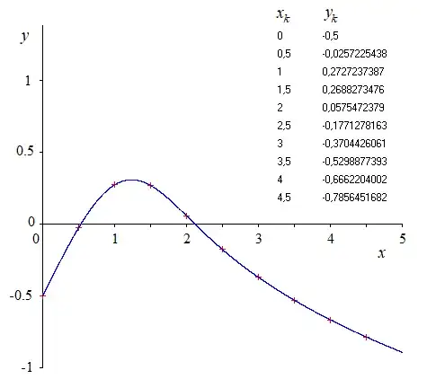
In addition, NUMERICAL EXAMPLE :

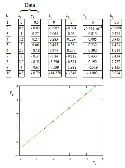
We observe that the $E_k(x_k)$ is quite linear as expected if the data approximately fits a solution of the differential equation. The linear regression gives $$E_k\simeq c_1\:x_k+c_2\quad\text{with } c_1=0.994\:;\: c_2=-0.517$$

After computing $c_1$ and $c_2$ it is possible to evaluate the initial conditions (at $x=x_1$) : $$y(x_1)=c_1x_1+c_2-\frac16 (x_1)^3\simeq y_1$$ $$y'(x_1)=c_1-(x_1)^2 y(x_1)-\frac12 (x_1)^2$$ For the above example the calculus was simplified because $x_1=0$ .

In fact, if the data was not approximate but exact and if the numerical integrations for $T_k,U_k,V_k$ were also exact, we should have found $c_1=1$ and $c_2=-0.5$

Of course all above doesn't gives the solution of the differential equation. Numerical methods and sofwares exist for solving the ODEs, given some conditions.

FOR INFORMATION :

The data was coming from the numerical solving of $y''+x^2y'+x=0$ with conditions $y'(0)=1$ and $y(0)=-0.5$ for example. Then rounded $y_k$ were taken as data to be used for the above numerical example.

Answer 2

We first need some way to estimate $k$:th derivative $d^ky/dx^k$ as Jacquelin mentions. There probably exist thousand ways to do this. Pick your favourite one.

Now we have data sets, for example $\{x,y,dy/dx,d^2y/dx^2\}$. We can create some arbitrary powerset of this. For simplicity just let $dy/dx$ be called $d$.

For example 2 degree polynomial: $$\{x,y,d,d^2,\\x^2,xy,xd,xd^2,\\yx,y^2,yd,yd^2,\\x^3,yx^2,x^2d,x^2d^2,\\xy^2,y^3,y^2d,y^2d^2\\x^2y,xy^2,xyd,xyd^2\}$$

You may see that the number of terms increase very fast.

This makes the use of some regularization more and more important the higher degree we use. Especially we want to be able to get sparse representation, for this a regularization norm of $<2$ or even $\leq 1$ is often desired. The last 10-15 years have seen growing popularity in $L_1$-norm regularizers. The solution is a vector of coefficients to the above data. The reason for the use of these norms in regularization is that we can get a sparse solution. This simplifies the model considerably. It is much nicer to have a model with say for example 3-4 terms (with non-zero coefficients) and some slightly larger error than a model with 24 terms and smaller error.