Gaussian 2-D Mixture, mean mode median of marginals and 2-D

Question

Let

p(x1,x2) = $\dfrac {4}{10}\mathcal{N}\left( \begin{bmatrix} 10 \\ 2 \end{bmatrix},\begin{bmatrix} 1 & 0 \\ 0 & 1 \end{bmatrix}\right) + \dfrac {6}{10} \mathcal{N}\left( \begin{bmatrix} 0 \\ 0 \end{bmatrix},\begin{bmatrix} 8.4 & 2.0 \\ 2.0 & 1.7 \end{bmatrix}\right)$ be a mixture of two gaussians.

a. Compute the marginal distributions for each dimension.

b. Compute the mean, mode and median for each marginal distribution.

c. Compute the mean and mode for the two-dimensional distribution.

---

I find this problem confusing, my approach for a.) I've used the fact p(x1) = $\mathcal{N}\left(x1|\mu_{x1},\sum _{11} \right)$

and a formula for the 1-D mixture: $p\left( x\right) =\alpha p_{1}\left( x\right) +\left( 1-\alpha\right) p_{2}\left( x\right)$

$\mu _{x}=\alpha\mu _{1}+ \left( 1-\alpha\right) \mu_{2}$ and $\sigma = \alpha \left( \mu ^{2}_{1} + \sigma^{2}_{1} \right) + (1-\alpha)\left( \mu ^{2}_{2} + \sigma^{2}_{2} \right)$

to achieve $\mu_{x1} = 4/10.10+0.6.0 = 4 $

and $\sum _{11} = 0.4(10^{2}+1) + 6/10(0+8.4^{2})$ =82.736

and similarly $\mu_{x2} = 0.8$ and $\sum _{22} = 3.734$

for part b) the mean mode and median should be the mean?

and part c) p(x1,x2) = $\mathcal{N}\left( \begin{bmatrix} \mu_{x1} \\ \mu_{x2} \end{bmatrix},\begin{bmatrix} \sum _{11} & \sum _{12} \\ \sum _{21} & \sum _{22} \end{bmatrix}\right)$ where I need to calculate the covariances.

I am sure this approach is not correct, any help would be appreciated as this problem is completely different to the others I have been working through.

Answer 1

Let $f_{X_1,Y_1}(x,y)$ and $g_{X_2,Y_2}(x,y)$ represent the densities for the joint random variables $$(X_1,Y_1) \sim \operatorname{Binormal}(\boldsymbol \mu_1, \boldsymbol \Sigma_1), \\ (X_2,Y_2) \sim \operatorname{Binormal}(\boldsymbol \mu_2, \boldsymbol \Sigma_2) $$ where $$\boldsymbol \mu_1 = \begin{bmatrix}10 \\ 2 \end{bmatrix}, \quad \boldsymbol \Sigma_1 = \begin{bmatrix}1 & 0 \\ 0 & 1 \end{bmatrix}, \\ \boldsymbol \mu_2 = \begin{bmatrix}0 \\ 0 \end{bmatrix}, \quad \boldsymbol \Sigma_2 = \begin{bmatrix}8.4 & 2.0 \\ 2.0 & 1.7 \end{bmatrix}$$ are the means and variance-covariance matrices. Then let $h_{X,Y}(x,y) = \frac{4}{10}f_{X,Y}(x,y) + \frac{6}{10}g_{X,Y}(x,y)$ be the mixture density of the joint random variables $X,Y$. We know the marginal distribution $$h_X(x) = \int_{y=-\infty}^\infty h_{X,Y}(x,y) \, dy = \frac{4}{10} \int_{y=-\infty}^\infty f_{X,Y}(x,y) \, dy + \frac{6}{10} \int_{y=-\infty}^\infty g_{X,Y}(x,y) \, dy = \frac{2 f_X(x) + 3 g_X(x)}{5}.$$ That is to say, the marginal density of $X$ is simply the corresponding mixture of the marginal densities $f$ and $g$, respectively, and these are straightforward to obtain in the general bivariate normal case, so we will not do the computation here. One should obtain $$h_X(x) = \sqrt{\frac{3}{560\pi}} e^{-5x^2/84} + \sqrt{\frac{2}{25\pi}} e^{-(x-10)^2/2}.$$ The marginal density for $Y$ follows a similar computation.

From the above, you would then compute the mean by integrating, or recognizing that you can weight the means of the mixture component densities. The medians and modes cannot be computed in closed form; a numeric approach is required. You should get $$\text{mode}[X] \approx 9.9983954749618305175, \\ \text{mode}[Y] \approx 1.3308014487646739409, \\ \text{median}[X] \approx 2.8038540773512769026, \\ \text{median}[Y] \approx 0.86864477748682360773.$$

Finally, the joint mode of $(X,Y)$ is again not computable in closed form; a numeric approach is required: $$\text{mode}[X,Y] \approx (9.9985480617596613783, 2.0003568284284785974).$$

Answer 2

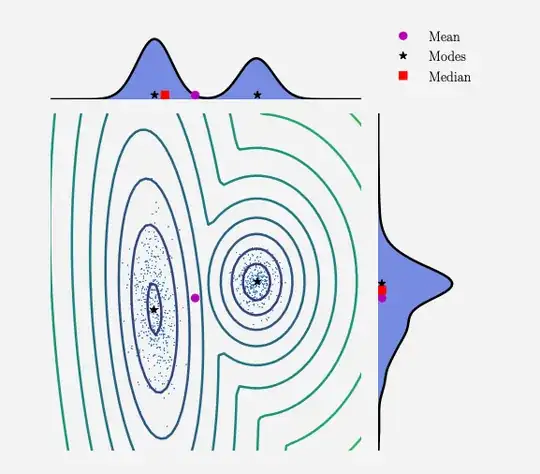
Neither the marginal distributions, nor the joint distributions are normal. Here's a picture from the book where this exercise is from (https://mml-book.github.io/):

I agree with @heropup approach of calculating marginal distributions analytically. I also agree that neither the marginal, nor the joint summary statistics can be computed analytically - you need to run a simulation, as distributions are not named.

What I got in my analysis:
Means for x,y: 4.0, 0.8
Medians for x,y: 8.0, 1.0
Modes for x,y (I bucketed into 100 buckets): 10,2

Intuitively all of the above seem to make sense to me.

Regarding joint statistics, isn't it just an array of marginal? So eg isn't the joint mean simply [4.0, 0.8]?

Answer 3

Your approach is correct for mean and incorrect for the variance. In fact you should have written $$\mu^2+\sigma^2=\alpha(\mu_1^2+\sigma_1^2)+(1-\alpha)(\mu_2^2+\sigma_2^2)$$therefore $$\mu_X=4\\\mu_X^2+\sigma_X^2=0.4(10^2+1^2)+0.6(0^2+8.4^2)=58.496\implies\\\sigma^2_X=42.496\implies \\X\sim\mathcal{N}(4,42.496)$$and$$\mu_Y=0.8\\\mu_Y^2+\sigma_Y^2=0.4(2^2+1^2)+0.6(0^2+1.7^2)=3.674\implies\\\sigma^2_Y=3.034\implies \\Y\sim\mathcal{N}(0.8,3.034)$$

b) The mean, mode and median are the same for a univariate Gaussian distribution by definition.

c) Note that the joint distribution $p(x,y)$ is NOT Gaussian itself.

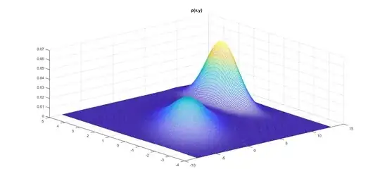
The mean is $\begin{bmatrix}4\\0.8\end{bmatrix}$ and the mode is $(x_0,y_0)$ such that$$(x_0,y_0)=\text{arg}\max_{(x,y)}p(x,y)$$ Now since $p(x,y)$ is $C^2[\Bbb R^2]$, in the extremal points we have $${\partial \over \partial x}p(x,y)={\partial \over \partial y}p(x,y)=0$$Define $$N_1\triangleq{1\over 2\pi}\exp\left(-{1\over 2}(x-10)^2-{1\over 2}(y-2)^2\right)$$and$$N_2={1\over 2\pi\cdot3.2062}\exp\left(-{1\over 2}[0.1654x^2+0.8171y^2-0.3892xy]\right)$$then the equations ${\partial \over \partial x}p(x,y)={\partial \over \partial y}p(x,y)=0$ lead to$${(x-10)N_1+0.0516xN_2=0\\(y-2)N_2+0.2549yN_1=0}$$The latter set of equations cannot be solved analytically, but numerically we obtain the following three candidates for the maximum$$(x_1,y_1)=(-0.0402,-0.0201)\\(x_2,y_2)=(10.0452,2.0151)\\(x_3,y_3)=(1.7227,6.6705)$$By checking the 2-nd order condition (again, numerically) we obtain $$(x_0,y_0)=\text{arg}\max_{(x,y)}p(x,y)=(10.0452,2.0151)$$therefore>$$\text{mode}=(10.0452,2.0151)$$you may observe the $3d$ graph of the $p(x,y)$ below