Let us derive the Kurganov-Tadmor central scheme for Burgers' equation $u_t + f(u)_x = 0$ which physical flux $f(u) = \frac{1}{2}u^2$ is convex. The numerical method is written in semi-discrete form (see Eq. (4.2) of (1))
$$
\frac{\text d u_i}{\text d t} = -\frac{H_{i+1/2} - H_{i-1/2}}{\Delta x} ,
$$
where the numerical flux reads
$$
\begin{aligned}
H_{i+1/2} &= \frac{1}{2} \left(f(u^L_{i+1/2}) + f(u^R_{i+1/2}) - a_{i+1/2}\, (u^R_{i+1/2}-u^L_{i+1/2})\right) ,\\
a_{i+1/2} &= \max \left\lbrace |f'(u^L_{i+1/2})|, |f'(u^R_{i+1/2})|\right\rbrace .
\end{aligned}
$$
The slope-limited extrapolated interface values of $u$ are given by
$$
\begin{aligned}
u_{i+1/2}^{L} &= u_i + \frac{\Delta x}{2} (u_x)_{i} ,\\
u_{i+1/2}^{R} &= u_{i+1} - \frac{\Delta x}{2} (u_x)_{i+1} ,\\
(u_x)_{i} &= \text{minmod}\left(\frac{u_i-u_{i-1}}{\Delta x}, \frac{u_{i+1}-u_{i}}{\Delta x}\right) ,
\end{aligned}
$$
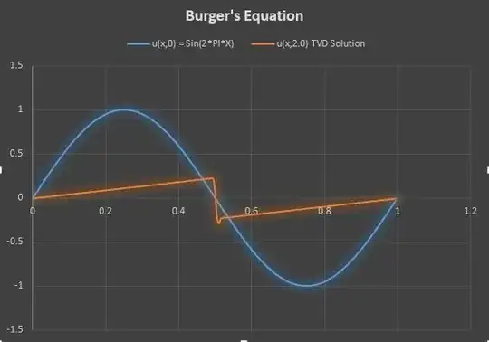
where the minmod limiter function is $(a,b)\mapsto \frac{1}{2}(\text{sign}\, a + \text{sign}\, b)\min(|a|,|b|)$. Numerical results obtained with the following piece of Matlab code are shown below. Here, second-order Runge-Kutta integration is used. The Courant number is set to $\text{Co} = 0.2$, and periodic boundary conditions are implemented. Numerically, it seems that TV-stability is even preserved for larger Courant numbers, e.g. $\text{Co} = 0.9$, but this is no longer true if forward Euler time-integration is used instead of the present RK2 method. Note that the modification $(u_x)_i = 0$ of the method yields the local Lax-Friedrichs (a.k.a Rusanov) method if forward Euler time-integration is used.
function y = minmod(a,b)
    y = 0.5*(sign(a)+sign(b)).*min(abs(a),abs(b));
end

function [y,yp] = f(u)
    y = 0.5*u.^2;
    yp = u;
end

function y = RHS(u,dx)
    ux = minmod((u-circshift(u,[0 1]))/dx,(circshift(u,[0 -1])-u)/dx);
    uL = circshift(u + 0.5*dx*ux,[0 1]);
    uR = u - 0.5*dx*ux;
    [fL,fpL] = f(uL);
    [fR,fpR] = f(uR);
    a = max(abs(fpL),abs(fpR));
    H = 0.5*(fL + fR - a.*(uR-uL));
    y = -(circshift(H,[0 -1]) - H)/dx;
end

%%%%%%%%%%%%%% main program %%%%%%%%%%%%%%
%parameters
Nx = 200;
Co = 0.2;
tmax = 2;

%initialization
x = linspace(0,1,Nx);
t = 0;
u = sin(2*pi*x);
dx = x(2) - x(1);
dt = Co*dx/max(abs(u));

figure(1);
clf;
plot(x,u);
hold on
h = plot(x,u,'k.');

%iterations
while (t<tmax)
    u1 = u + dt*RHS(u,dx);
    u = 0.5*u + 0.5*(u1 + dt*RHS(u1,dx));

    set(h,'YData',u);
    drawnow;

    dt = Co*dx/max(abs(u));
    t  = t + dt;
end
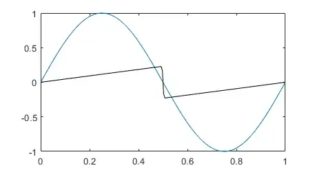
The theoretical solution can be obtained quasi-analytically by following the steps in this post. Indeed, a static shock is located at $x=0.5$, and the solution on each side can be deduced from the method of characteristics. Hence, we need to solve numerically the equation $u = \sin (2\pi (x - ut))$ to find the value of $u(x,t)$ at $x\neq 0.5$, which can be done by using root finding methods:
fun = @(u) u - sin(2*pi*(x-u*t));
u0 = x/t.*(x<0.5) + (x-1)/t.*(0.5<x);
uth = fsolve(fun,u0);
plot(x,uth,'r');
disp(norm(uth-u));
Repeating these steps for various mesh sizes $\Delta x$ leads to error measurements. However, it should be noted that we are limited by the precision of the root finding method. Lastly, the order of convergence equals $\approx 0.5$ when the solution is discontinuous (i.e., when $t>\frac{1}{2\pi}$ is larger than the breaking time).
(1) A. Kurganov, E. Tadmor (2000): "New High-Resolution Central Schemes for Nonlinear Conservation Laws and Convection-Diffusion Equations", J. Comput. Phys. 160(1), 241–282. doi:10.1006/jcph.2000.6459