2

I have written some python code which was designed to try to solve the following differential equation: $$\ddot{x}+\omega_0^2x=\eta(t),$$ where $\eta(t)$ is the gaussian white noise, with mean 0 and variance 1. The initial conditions are: $$x(0)=\dot{x}(0)=0.$$ The code is given here:

import numpy as np
import matplotlib.pyplot as plt
from scipy.stats import norm

class HarmonicOdeSolver:
    def __init__(self, dt, x0, xd0, omega_squared):
        "Inits the solver."
        self.dt = dt
        self.dt_squared = dt ** 2
        self.t = dt
        self.omega_squared = omega_squared
        self.x0 = x0
        self.xd0 = xd0
        self.x = [xd0 * dt + x0, x0]

    def step(self):
        "Steps the solver."
        xt, xtm1 = self.x
        xtp1 = (2 - self.omega_squared * self.dt_squared) * xt - xtm1 \
             + self.dt_squared * norm.rvs()
        self.x = (xtp1, xt)
        self.t += self.dt

    def step_until(self, tmax, snapshot_dt):
        "Steps the solver until a given time, returns snapshots."
        ts = [self.t]
        vals = [self.x[0]]
        niter = max(1, int(snapshot_dt // self.dt))
        while self.t < tmax:
            for _ in range(niter):
                self.step()
            vals.append(self.x[0])
            ts.append(self.t)
        return np.array(ts), np.array(vals)

solver = HarmonicOdeSolver(1e-2, 0, 0, 1)
snapshot_dt = 1.0
ts, vals = solver.step_until(1000, snapshot_dt)
plt.plot(ts, np.sqrt(vals ** 2))
plt.plot(ts, np.sqrt(ts / 2))

The code was taken from and explained here. I naively hoped that I could simply add the following line of code:

self.dt_squared * norm.rvs()

to simulate Gaussian white noise. One problem I have noticed is that the results appear to be highly dependent on the time step used. In a similar post we found that the variance of the oscillator should grow as: $$\sqrt{\langle x(t)^2\rangle}\sim\sqrt{\frac{t}{2}}.$$ I would like to reproduce this result, does anyone know of a simple way to simulate a harmonic oscillator driven by white noise?

EDIT: Thanks for the help WoofDoggy, however, I am still confused. When you turned the ODE into a system of stochasic differential equations should you have not done this: $$dX_t=\dot{X}_tdt,$$ $$d\dot{X}_t=-\omega_0^2X_tdt+dW_t,$$ but instead you have done this: $$dX_t=\dot{X}_tdt+dW_t,$$ $$d\dot{X}_t=-\omega_0^2X_tdt?$$
Peanutlex
  • 1,169

1 Answers1

2

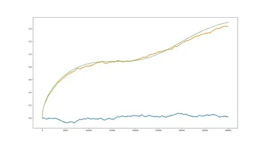
What you are dealing with is called stochastic differential equation. Go back to the differential form: $$ \mathbf{X}_t = \left[\begin{array}{c} X_t \\ \dot{X}_t \end{array} \right],$$ and write down the equation in matrix form $$d\mathbf{X}_t = \mathbf{M} \cdot \mathbf{X}_t dt + \left[\begin{array}{c}dW_t\\0\end{array}\right],$$ where $dW_t = \eta(t)dt$ and $\mathbf{M} = \left[\begin{array}{cc}0 & 1 \\ -\omega_0^2 & 0\end{array} \right]$. Now you can numerically simulate the process using Euler-Maruyama method: $$\mathbf{X}_{t+1} = \mathbf{X}_t + \mathbf{M} \cdot \mathbf{X}_t \Delta t + \left[\begin{array}{c}\Delta W_t\\0\end{array}\right],$$ and keep in mind that $\Delta W_t$ is a Gaussian random variable (with parameters mentioned in the question). If your discretization domain is small enough and you collected enough samples you should see a plot similar to the one below. Blue line is the mean $\langle X_t\rangle$ and orange $\sqrt{\langle X_t^2 \rangle}$.

enter image description here

EDIT

A little bit of theoretical explanation. The solution can be written as $$\mathbf{X}_t = e^{t \mathbf{M}} \mathbf{X}_0 + \int\limits_{0}^{t} e^{-(s-t)\mathbf{M}} \left[\begin{array}{c}\eta(s)\\0\end{array}\right]ds.$$ Since $\mathbf{X}_0 = \mathbf{0}$, we can write $$X_t = \frac{1}{\omega_0}\int\limits_{0}^{t} \cos[\omega_0(s-t)] \eta(s)ds$$ and you get (for $\omega_0 = 1$) $$\langle X_t^2\rangle = \frac{1}{2}t + \frac{\sin(2t)}{4}$$

SAMPLE Python code

# -*- coding: utf-8 -*-
import numpy as np

def run(x0=np.array([.0,.0]), n=40000, dt=1.0E-04, omega=1.0):

    sol = np.array([])

    M = np.array([[0, 1.],[-omega**2, 0.]])

    x = x0.copy()
    for i in range(0,n):
        sol = np.append(sol, x[0])
        x += M @ x * dt + np.array([1.,0.]) * np.random.normal(scale=np.sqrt(dt))


    return sol

sol = np.array([run() for i in range(0,500)])

mean  = np.mean(sol, axis=0)
sigma = np.sqrt(np.var(sol, axis=0) + mean**2)

dt = 1.0E-04
x = np.arange(0, len(mean))
y = np.sqrt(x * dt/2. + np.sin(2. * x * dt)/4.)

import matplotlib.pyplot as plt

fig, ax = plt.subplots(figsize=(15,10))


ax.plot(x, mean)
ax.plot(x, sigma)
ax.plot(x, y)
plt.show()
WoofDoggy
  • 379
  • Thank you, do you mind posting the code you used? – Peanutlex Dec 30 '18 at 18:14
  • Thanks. Shouldn't the final value of $\sqrt{\langle X_t^2\rangle}$ be $1/\sqrt{2}$? Also, the following equation does not make sense to me:$$d\textbf{X}_t=\textbf{M}\cdot\textbf{X}_tdt+[dW_t,0],$$ as this would mean the second element of the vector would be: $$d^2X_t=-\omega_0^2X_tdt,$$ but surely it should reduce to:$$d^2X_t/dt=-\omega_0^2X_tdt+dW_t?$$ Finally, have you made a mistake in your code at line 13, should it be: np.random.normal(scale=dt)? – Peanutlex Dec 30 '18 at 20:35
  • Sorry, should the code be: np.random.normal(scale=np.sqrt(dt))? – Peanutlex Dec 30 '18 at 20:45
  • @Peanutlex yes, my bad. The plot will change then. – WoofDoggy Dec 30 '18 at 20:46
  • Thanks a lot. Do you mind showing how you derived this equation:$$d\textbf{X}_t=\textbf{M}\cdot\textbf{X}_tdt+[dW_t,0]?$$ – Peanutlex Jan 03 '19 at 11:35