How to solve $u_t + uu_x =\delta(x)$

Question

I am studying from old exams and there is a problem which is traffic flow with a ramp.

I have never seen this type of problem in class, so for the simple case, how would I solve $$u_t + uu_x =\delta(x)\\ u(0,x) = 1$$ with method of characteristics.

I think we have $$\frac{dt}{ds} = 1 \quad \text{ with } t(0) = 0$$ $$\frac{dx}{ds} = u(s) \quad \text{ with } x(0) = x_0$$ $$\frac{du}{ds} = \delta(x(s)) \quad \text{ with } u(0) = 1$$ From these, I can get $$\frac{d^2x}{ds^2} = \delta(x(s))$$ and how would I continue?

Further attempt: Now we pick some $x(0) = x_0 \neq 0$ as the initial condition for $$\frac{d^2x}{ds^2} = \delta(x(s))$$ Now we assume that $x$ is continuous, so in a short time, $x(s) \neq 0$ for $0<s<S$, this means we have $$\frac{du}{ds} = 0\quad\quad \frac{dx}{ds} = u(s)=u(0) = 1$$ so we get the solution $x(s) = 1\cdot s + x_0$. Next we see that when $x_0<0$, after time $s=|x_0|$, $x$ will become zero, this means there will be a jump in the value of $u$, and after the jump, $u$ will take the constant value $1+1 = 2$, $1$ from the initial value, $1$ from the dirac. Then the characteristics we have $x(s) = 2\cdot s - 2\cdot|x_0|$ for $s>|x_0|$.

Is this approach okay?

Answer 1

Let us represent the Dirac delta by $\displaystyle\delta(x) = \lim_{\varepsilon\to 0^+} \eta_\varepsilon(x)$, where $$ \eta_\varepsilon(x) = \frac{1}{\varepsilon}\text{rect}\left(\frac{x}{\varepsilon}\right) = \left\lbrace \begin{aligned} &{1}/{\varepsilon}\, , & & {-\varepsilon}/{2} < x < {\varepsilon}/{2}\\ &0\, , & &\text{otherwise} \end{aligned} \right. $$ is a rectangular function. We consider the Cauchy problem $u_t + u u_x = \eta_\varepsilon(x)$ with initial data $u(x,0) = 1$ for some $\varepsilon>0$.

For all abscissas $x_0$, the initial data is $u(x_0,0) = 1$. If $\varepsilon\to {+\infty}$, the (homogeneous) inviscid Burgers' equation is recovered. In this limit case, the characteristics are straight lines with slope 1 in the $x$-$t$ plane along which $u$ is constant. Now, we consider $\varepsilon<+\infty$. The first part of the method of characteristics gives ${\text d t}/{\text d s} = 1$. Letting $t(0)=0$, we know $t=s$. The other part reads $$ \left\lbrace\begin{aligned} \frac{\text d x}{\text d s} &= u(s)\\ \frac{\text d u}{\text d s} &= \frac{1}{\varepsilon}\text{rect}\left(\frac{x(s)}{\varepsilon}\right) \end{aligned}\right. $$ where $u(0)=1$ and $x(0)=x_0$. Several cases are examined:

1. If $x_0\geq\varepsilon/2$, we start with $\text{rect}(x_0/{\varepsilon})=0$. Therefore, we know $u=1$ and $x=x_0+t$ for all $t$.

2. If $-\varepsilon/2<x_0<\varepsilon/2$, we start with $\text{rect}(x_0/{\varepsilon})=1/\varepsilon$. Therefore, we know $u=1+{t}/{\varepsilon}$ and $x=x_0+t+{t^2}/(2{\varepsilon})$ up to $t = t_1 = \varepsilon\left(\sqrt{2\left(1- x_0/\varepsilon\right)}-1\right)$, where $x=\varepsilon/2$. For $t > t_1$, we have again straight lines with equation $x = \varepsilon/2 + u_1\left(t - t_1\right)$, along which $u$ is constant and equal to $u_1 =\sqrt{2\left(1- x_0/\varepsilon\right)}$.

3. If $x_0\leq-\varepsilon/2$, we start with $\text{rect}(x_0/{\varepsilon})=0$. Therefore, we know $u=1$ and $x=x_0+t$ up to $t=t_1=-\varepsilon/2-x_0$, where $x=-\varepsilon/2$. From $t = t_1$, we have again $u=1+({t}-t_1)/{\varepsilon}$ and $x=-\varepsilon/2+t-t_1+{(t-t_1)^2}/(2{\varepsilon})$ up to $t = t_2 = t_1 + \left(\sqrt{3}-1\right)\varepsilon$, where $x=\varepsilon/2$. For $t > t_2$, we have again straight lines with equation $x = \varepsilon/2 + u_2\left(t - t_2\right)$, along which $u$ is constant and equal to $u_2 =\sqrt{3}$.

In the figure below, we represent the characteristics so-obtained for $\varepsilon = 1/2$:

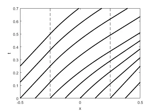
The characteristic curve $x = \varepsilon/2 + t$ intersects a characteristic curve coming from $]-\varepsilon/2,\varepsilon/2[$ at $(x_b,t_b) = (\frac{3}{2}\varepsilon,\varepsilon)$. Hence, a shock wave is generated. On the right of the shock, the data is $u=1$. As long as the left data comes from $]-\varepsilon/2,\varepsilon/2[$, we have $t_1 = t - ({x_s-\varepsilon/2})/{u_1}$ and $t_1 = \varepsilon \left(u_1-1\right)$, which gives the data $u = u_1$. The abscissa $x_s$ of the shock satisfies the Rankine-Hugoniot condition $x'_s(t) = \frac{1}{2}\left(1 + u_1\right)$ with initial condition $x_s(\varepsilon) = \frac{3}{2}\varepsilon$, i.e. \begin{aligned} x'_s(t) &= \frac{1}{2}\left(1 + \frac{1+t/\varepsilon}{2}\left(1 + \sqrt{1 + 2\frac{\varepsilon-2x_s(t)}{1+t/\varepsilon}}\right) \right) \\ &\simeq 1+\frac{t}{2\varepsilon} + \frac{\varepsilon-2x_s(t)}{4} \end{aligned} which provides an approximation of $x_s(t)$.

To solve the full problem, one must consider also the case where the left data comes from $]-\infty,-\varepsilon/2[$, and then take the limit as $\varepsilon\to 0^+$.

---

The traffic flow problem with the ramp may be related to this post.

Answer 2

From your characteristic equations you can swap $s$ for $t$ (i.e. find $x(t)$ and $u(t)$ such that $u(x(t),t)=u(t)$) and you are left with having to solve $$ u'(t)=\delta(x(t)) \\x'(t)=u(t) $$ Where $x(t)\neq 0$, you get $u=\text{const}=u_0$, and so $x(t)=x_0+u_0t$. If $x_0 > 0$, these lines are diagonal, $u_0=1$ due to the initial condition and they continue for every like this unperturbed. If $x_0<0$, these lines are initially also diagonal, i.e. $u_0=1$ until they cross the $x=0$ line at $t=t_0=-x_0>0$. After the characteristics have crossed the $x=0$ line, they will continue with a constant speed again (because away from $x=0$, $u=\text{const}$ again), but this speed will have a distinct value, say $u_+ \neq 1$, because there will be a jump in $u$ at $x=0$ induced by the Dirac term. (Make a drawing, it will be clear. I think that was your intuition as well.)

To determine the size of the jump in $u$ at $x=0$, we integrate the equations above over $s\in(t_0-, t_0+)$, where $t_0\pm=t_0\pm \epsilon$ for $\epsilon > 0, \epsilon\to 0$, and $t_0=-x_0$ is the time at which the characteristic encounters the ramp ($x=0$). Assuming that $u(s)$ is bounded by $M>0$, integrating the second equation and taking the absolute value gives $|x(t_0+)-x(t_0-)|=|\int_{t_0-}^{t_0+}dt\,u(t)|\leq \int_{t_0-}^{t_0+}dt\,|u(t)|\leq 2 M \epsilon\to 0$ by Lebesgue theorem of dominated convergence, which shows that $x(t)$ is continuous at $t=t_0$ as expected.

Integrating the first equation should give the jump in $u(t)$ at $t=t_0$. The problem is that $x(t)$ is not smooth at $t=t_0$ (slope change), but let's go on for a bit just to see: for a function $x(t)$ with a single zero at $t=t_0$, one has $\delta(x(t)) = \frac{\delta(t-t_0)}{|x'(t_0)|}$, so that $$ \int_{t_0-}^{t_0+}dt\,u'(t) = u(t_0+)-u(t_0-) = \int_{t_0-}^{t_0+}dt\,\delta(x(t)) = \int_{t_0-}^{t_0+}dt\frac{\delta(t-t_0)}{|x'(t_0)|}=\frac{1}{|u(t_0)|} $$ The problem here is clear: the size of the jump in $u(t)$ at $t=t_0$ is ill-defined in this formula: $u(t_0)$ doesn't have a value. I think that the trick to get rid of this problem goes as follows. Assuming $u(t)>0$, rewrite $$ u'(t)=\delta(x(t))=\frac{\delta(t-t_0)}{|x'(t_0)|}=\frac{\delta(t-t_0)}{|x'(t)|} \implies u(t)u'(t) = \delta(t-t_0) \\\implies \frac{d}{dt}u^2(t) = 2\delta(t-t_0) $$ Now integrating this equation instead gives $u^2(t_0+)-u^2(t_0-)=2$ and so $u(t_0+)=u_+=\sqrt{3}$. The characteristics that cross the $x=0$ line will instantaneously change their slope from 1 to $u_+ = \sqrt{3}>1$, and will therefore collide with the characteristics that left with $x_0>0$ (shock formation). It's probably worth checking that this procedure will indeed give you a solution that solves the initial problem...

Answer 3

Let us write the corresponding Rankine-Hugoniot condition. Consider that $u$ has a single discontinuity with jump $u^+-u^-$ at $x=\gamma(t)$ between $x_1$ and $x_2$. Since $u$ is nonsmooth, we go back to the integral definition of the conservation law $$ \frac{\text d}{\text d t} \int_{x_1}^{x_2} u\,\text d x = \left\lbrace\begin{aligned} &\tfrac12 u^2|_{x=x_1} - \tfrac12 u^2|_{x=x_2} & &\text{if}\quad 0 \notin [x_1,x_2] \\ &\tfrac12 u^2|_{x=x_1} - \tfrac12 u^2|_{x=x_2} + 1 & &\text{if}\quad 0 \in [x_1,x_2] \end{aligned}\right. $$ Then, the identity $$ \frac{\text d}{\text d t} \int_{x_1}^{x_2} u\,\text d x = \int_{x_1}^{\gamma(t)} u_t\,\text d x + \int_{\gamma(t)}^{x_2} u_t\,\text d x + \gamma'(t)\left(u^--u^+\right) $$ and the PDE yield the modified Rankine-Hugoniot condition $$ \left\lbrace\begin{aligned} \gamma'(t) &= \tfrac12 (u^+ + u^-) & &\text{if}\quad \gamma\neq 0 \\ 0 &= \tfrac12 (u^+ + u^-) - {(u^+-u^-)}^{-1} & &\text{if}\quad \gamma = 0 \end{aligned}\right. $$ as $x_2 \to x_1$. The solution to the initial-value problem has two discontinuities:

• At $x = 0$, we have a static discontinuity with left state $u^- = 1$ and right state $u^+ = \sqrt{3}$.
• At $x = st$ with $s = \frac12 (1 + \sqrt{3})$, we have an admissible shock wave with left state $u^- = \sqrt{3}$ and right state $u^+ = 1$.

Hence, $$ u(x,t) = \left\lbrace\begin{aligned} & 1 & &\text{if}\quad x<0 \\ &\sqrt{3} & &\text{if}\quad 0 < x < \tfrac{1 + \sqrt{3}}2 t \\ & 1 & & \text{if}\quad x>\tfrac{1 + \sqrt{3}}2 t \end{aligned}\right. $$