3

Robust line fitting to a set of 2D points is a well studied problem for which several approaches are known. They usually consider the point cloud as unstructured.

I call a digital path a sequence of pixels (points with integer coordinates) that are 8- or 4- connected. We may assume that the abscissa grows monotonously.

I wan to fit a line segment to a given path, in such a way that the deviations from the segment do not exceed a given threshold (a few pixels), while the segment is the longest possible.

Any hint ?

enter image description here

I am well aware of the Douglas-Peucker algorithm, but it is not suitable to find a single segment.


Update:

By means of the Melkman algorithm, we can compute the convex hull from one endpoint toward the other, in linear time N) for N pixels. From the convex hull, the minimum width can be obtained by Rotating Calipers, in time linear wrt the hull size. This would yield a total O(NH) effort to compute all widths (H pixels on the hull on average). But I suspect that the Rotating Calipers could be applied incrementally, starting from the previous position on the previous hull, resulting in a better amortized complexity. I didn't prove this formally.

Equipped with this device, we can find sections out of tolerance. But this doesn't tell us yet how to find the longest one.


Next Update:

Using a dynamic convex hull algorithm, it should be possible to let the hull grow by adding vertices in path order, until the width exceeds the given tolerance. Then remove an initial vertex, and add end vertexes until the tolerance is exceeded again, and so on.

This way, in a number of hull updates that is linear in the number of vertexes, we can find all parts of the path that are just below the tolerance. By combining with the previous idea (Rotating Calipers update upon hull update), I guess that an efficient solution can be achieved.
3 Answers3

1

This is not a full answer to the question, but a related piece of information.

The algorithms used to solve this kind of problems involve iterative calculus generally requiring initial guess.

The method shown below is direct, without iteration and so, without initial guess. The general principle is explained in the paper : https://fr.scribd.com/doc/14674814/Regressions-et-equations-integrales

For the application to the present problem, the theory has to be extended to the case of piecewise functions, which is not published in the 2013 edition of the paper referenced above (See the updated answer below). The calculus process is presented in the next page :

enter image description here

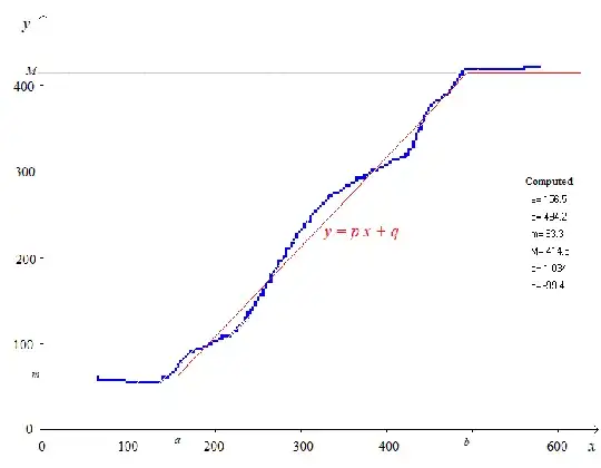
The results are the parameters $p$ , $q$ of the equation of the segment $y(x)=px+q$ as well as the coordinates of the two break points $(a,m)$ and $(b,M)$ .

A numerical example with all calculus steps is added in order to check the correct writing of the code.

enter image description here

APPLICATION to the figure given in the question :

Adding the axes and scanning a copy of the figure gave the data of the coordinates of the pixels. Then, the calculus according to the above method leads to the result shown on the next figure :

enter image description here

The fitted piecewise function is drawn in red.

Note that in this method, the criteria of fitting is not one among the criterion usually considered, which can be of various kind, leading to different results according to minimum MSE or RMSE or MAE, etc. In fact it is the fitting of an integral equation which solution is the sought piecewise function. As a consequence, it is not surprising that the result be slightly different from the results of more common methods.

If a criteria of fitting is strictly specified, the above method is not convenient, but it can provide an accurate initial start (instead of a guess) for some iterative process.

UPDATED ANSWER :

A provisional version of a new paper about piecewise regression is now published on : https://fr.scribd.com/document/380941024/Regression-par-morceaux-Piecewise-Regression-pdf

The present case of function made of three straight line segments is given pages 17-19.

In this late paper, a slightly different integral equation, but equivalent, is considered with the advantage of simpler numerical integrations. The numerical results for the Yves Daoust's example are so close from the preceding ones that it's not worthwhile to re-edit the results. Only the algorithm has been updated.

JJacquelin
  • 68,401
  • 4
  • 40
  • 91
  • Interesting. Does that generalize to more pieces, where the number of pieces is unknown ? Piecewise fitting problems with unknown knots are notably difficult. –  May 18 '18 at 10:07
  • Yes, in theory this can be generalised to more pieces with unknown knots. But I am afraid that would be more and more difficult in practice. In the present case, we have four adjustable parameters because two segments are horizontal. With three arbitrary segments, we have 6 parameters. And two more parameters for each more segments. – JJacquelin Jun 04 '18 at 14:22
  • In fact, I delete my previous comment which was too pessimistic. Your question gave me the opportunity to comme back to a paper left uncompleted some years ago. After looking again at what was already done, I see that important simplifications occur in the case of piecewise function made of straight line segments. So I decided to publish the available stuff, while it is far to be completed : https://fr.scribd.com/document/380941024/Regression-par-morceaux-Piecewise-Regression-pdf – JJacquelin Jun 04 '18 at 14:31
0

$\mathbf{\color{brown}{\text{Preliminary scheme}}}$

Let $$\mathbb M = \{M_i(x_i,y_i),\quad i = 1,2,\dots, N\}\tag1$$ is the issue set of points (pixels).

Let $$\mathbb P = \{P_{i,j}(M_i, M_j),\quad i < j\}\tag2$$ is the set of lines, and let $$k(P_{i,j})=k_{i,j} = (\mathrm {slope}(P_{i,j}),\quad b(P_{i,j})= b_{i,j} = \mathrm{intercept}(P_{i,j}))\tag3$$ are the vectors of the slopes and the intercepts for the set of lines.

Let $$\mathbb C_l=\{C_iC_j\in \mathbb C_l\rightarrow \bigl(C_iC_j\in \mathbb P\bigr) \wedge \bigl(\forall (M_{k}\in\mathbb M) k_{i,j}x_k+b_{i,j} \le0\bigr),\}\tag4$$ $$\mathbb C_r=\{C_iC_j\in \mathbb C_r\rightarrow \bigl(C_iC_j\in \mathbb P\bigr) \wedge \bigl(\forall (M_{k}\in\mathbb M) k_{i,j}x_k+b_{i,j}\ge 0\bigr)\}\tag5$$ are the "convex" subsets of $\mathbb P,$ such that all the other points lie on one side of these straight lines or belongs to them.

CL and CR

$\mathbb C_L$ and $\mathbb C_R$ defines the sets of the left bound points $\mathbb P_L$ and the right bound points $\mathbb P_R,$ and that allow to eliminate from the search all another points.

Then one of the sets $$\mathbb S_L = \{k(C_{i,j}),\quad C_{i,j}\in \mathrm C_L\},\tag6$$ $$\mathbb S_R = \{k(C_{i,j}),\quad C_{i,j}\in\mathbb C_R\}\tag7$$ contains the slope of the optimal line.

If to use the line from $\mathbb C_L$ as the left bound line and "the most right" lines (with the "left" slope, passing through the "right" points from $\mathbb P_R$), as the right bound line, this provides half of the possible optimal variants.

Symmetric variant, with $C_R$ and $\mathbb P_L,$ leads to the other possible optimal variants.

Proposed scheme allows essentially decrease the search volume.

$\mathbf{\color{brown}{\text{The algorithm, details and complexity}}}$

$1.$ To form the boundary simplex, using the convex hull algoritm and to divide it to the left (L points) and right (R points) piecewize boundary parts.

Complexity: $O(N \ln N).$

$2.$ Using Fibonacci extrema searching, to find the segment of the left boundary having the least distance from the most far point of the right boundary (also using Fibonacci technique).

Complexity: $O(\log L\log R).$

$3.$ If the least distance is more than given, to use binary search method for the calculation of the quantities of non-used points.

Complexity (with p. $2$): $O(\log^2 L\log^2R).$

$4.$ To repeat pp. $4-5$ for the segments of the right boundary and the points of the left boundary.

Complexity (with p. $2$): $O(\log^2 L\log^2R).$

$5.$ To choose left or right segment and to build the line, which is parallel to segment and has the same distances from the segment and from the point.

$\mathbf{Note}.$ Realization of p.2 uses the unimodality of the searching functions on the simplex.

Pang
  • 407
  • 5
  • 9
  • I am not sure to understand your definitions. If an element of $\mathbb C$ must have all points of $\mathbb M$ on the same side, there is just about one such line. If only the points between the endpoints are concerned, then every pair of points in a concave section will do and the benefit is marginal (only halving of the number of possible lines). –  May 16 '18 at 14:32
  • @YvesDaoust $\mathbb C_L, \mathbb C_R$ consists only of the boundary lines and their points. – Yuri Negometyanov May 16 '18 at 16:34
  • @YvesDaoust First, we construct a convex left boundary and a convex right boundary and use only these points. Secondly, we use only those slopes that relate to the links of these boundaries – Yuri Negometyanov May 16 '18 at 16:47
  • Sorry, I even less understand now. –  May 16 '18 at 17:11
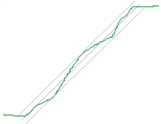
  • @YvesDaoust Added a graph with dots.Let us consider that the issue points set lays from one side of the every bound line. – Yuri Negometyanov May 16 '18 at 19:58
  • Your figure doesn't match my problem (there is no ordering among your points), and there is no guarantee that the directions defined by the green/blue points are related to the solution in any way. I am not after the width of a point cloud, which I know very well how to get in linear time. –  May 17 '18 at 07:37
  • @YvesDaoust Detalized MathCad illustration added. There are two main ideas: 1) we can consider only the points of the convex piecewise-linear boundary, and 2) the optimal solution should use left or right boundary slope. – Yuri Negometyanov May 17 '18 at 07:46
  • Sorry, I don't think you understood the problem. –  May 17 '18 at 07:50
  • @YvesDaoust The convex boundary building is well-known procedure. And all the other works quicker. – Yuri Negometyanov May 17 '18 at 07:53
  • @YvesDaoust Try to analyze how the green lines were built. The answer of the task is the middle line between them. – Yuri Negometyanov May 17 '18 at 08:02
  • No, you don't take into account the maximum deviation information. –  May 17 '18 at 08:41
  • @YvesDaoust Thanks, fixed. Waiting for comments. – Yuri Negometyanov May 17 '18 at 09:51
  • I already commented on your steps 1-2, which can be implemented in time O(N). Your explanations for 3-4-5 are too terse, and you still seem not to consider a sequence of points. –  May 17 '18 at 09:55
  • @YvesDaoust The estimation for the step $1$ can not be improved. The step 2 has the logarithmic complexity. – Yuri Negometyanov May 17 '18 at 09:59
  • Step 1 is performed in time O(N). You didn't read my post. Step 2 can be done in a straight way in time O(H), which is at worse O(N) and this is good enough. –  May 17 '18 at 10:05
  • @YvesDaoust Step $1$ is over the discussion. – Yuri Negometyanov May 17 '18 at 11:01
0

Using a dynamic convex hull algorithm, it should be possible to let the hull grow by adding vertices in path order, until the width exceeds the given tolerance. Then remove an initial vertex, and add end vertexes until the tolerance is exceeded again, and so on.

This way, in a number of hull updates that is linear in the number of vertexes, we can find all parts of the path that are just below the tolerance. By combining with the previous idea (Rotating Calipers update upon hull update), I guess that an efficient solution can be achieved.