Suppose a fair die is rolled $n = 60$ times, then the number $X$ of Ones seen
is $X \sim \mathsf{Binom}(n=60, p = 1/6).$ The expected number of Ones seen
is $E(X) = np = 60(1/6) = 10.$ The probability of seeing exactly 10 Ones
is $$P(X = 10) = {60 \choose 10}\left(\frac 1 6\right)^{10} \left(\frac 5 6\right)^{50} = 0.1270131.$$
PDF: The binomial PDF (or PMF) is defined as
$f_X(k) = {n \choose k}p^k(1-p)^{n-k},$ for $k = 0, 1, \dots, n.$ In R statistical software, $f_X(10),$ for $n=60,\, p=1/6,$ can be computed by using the displayed formula or by using
the built-in PDF dbinom:
choose(60,10)*(1/6)^10*(5/6)^50
[1] 0.1370131
dbinom(10, 60, 1/6)
[1] 0.1370131
CDF: The CDF is defined as
$F_X(k) = P(X \le k),$ for any real value of $k.$ In our example for $k < 0,$ we have
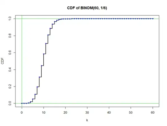
$F_X(k) = 0$ and for $k > n = 60,$ we have $F_X(k) = 1.$ From $k=0$ through $60,$ the CDF (denoted pbinom in R) is a 'pure jump' function, which can be plotted as shown below:
ml="CDF of BINOM(60, 1/6)"
curve(pbinom(x, 60, 1/6), -.5, 60.5, lwd=2, ylab="CDF", xlab="k", main=ml, n=10001)
abline(h=0:1, col="green3");  abline(v=0, col="green3")
k = 0:60; cdf=pbinom(k, 60, 1/6); points(k, cdf, pch=20, col="blue")
Blue dots emphasize that the value of the function $F_X(k)$ is the upper
end of each vertical segment.
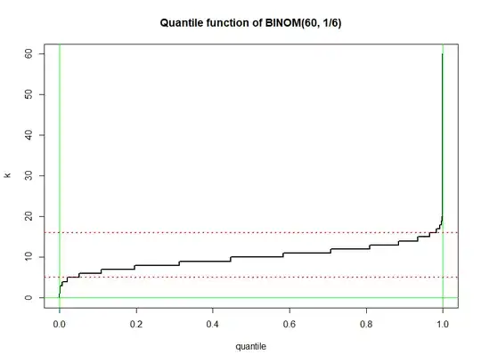
Inverse CDF: The 'quantile function' of $\mathsf{Binom}(60, 1/6)$ is the inverse of the CDF. In general, $F_X^{-1}(q) = c$ means $P(X \le c) = F_X(c) = q,$ for $0 < q < 1.$
In our example, the quantile function of $X$ can be used to get an interval in which values of $\mathsf{Binom}(60, 1/6)$
will lie with probability (just barely over) 95%. Specifically, $P(5 \le X \le 16)
= P(X \le 16) - P(X \le 4) = 0.96.$ (Because of the discreteness of the
binomial distribution it is not possible to get probability 0.95 exactly.)
qbinom(c(.025,.975), 60, 1/6)
[1]  5 16
diff(pbinom(c(4,16), 60, 1/6))
[1] 0.9633622
The plot of the quantile function is shown below with horizontal dotted
lines at 5 and 16:
ml = "Quantile function of BINOM(60, 1/6)"
curve(qbinom(x, 60, 1/6), 0, 1, lwd=2, n=10001, ylab="k", xlab="quantile", main=ml)
abline(v=0:1, col="green2");  abline(h = 0, col="green2")
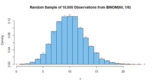
Using the quantile function to simulate a random sample: Finally, you can use the quantile function to simulate values of $X \sim \mathsf{Binom}(60, 1/6)$ from values of $U \sim \mathsf{Unif}(0,1).$
Below we use 10,000 standard uniform random variables to simulate as
many values of $X,$ for which $\bar X \approx E(X) = 10.$ (Notice that values of $X$ above about 20 or 25 are very rare.)
set.seed(518);  m = 10000;  u = runif(m);  x = qbinom(u, 60, 1/6;  mean(x)
[1] 9.9993  # aprx E(X) = 10
summary(x)
   Min. 1st Qu.  Median    Mean 3rd Qu.    Max.
  1.000   8.000  10.000   9.999  12.000  23.000
quantile(x, .999)
99.9%
   20
Below is a histogram of the simulated random sample of 10,000
observations from $\mathsf{Binom}(60, 1/6);$ centers of superimposed
open circles show exact binomial probabilities. (The fit is about
as good as can be anticipated for a sample of 10,000; a sample of a
million values would give a much better match.)
ml="Random Sample of 10,000 Observations from BINOM(60, 1/6)"
hist(x, prob=T, br=(min(x):(max(x)+1))-.5, col="skyblue2", main=ml)
  k=0:25; pdf = dbinom(k, 60, 1/6)
  points(k, pdf, col="red")
Notes: (a) If you use the same seed (in set.seed) as mine for the pseudorandom
number generator in R, you will get exactly the same 10,000 observations
I did. If you set a different seed, your results may be a little
closer to (or farther from) a perfect fit than mine. [If you set no seed,
R will pick an undisclosed, unpredictable seed from the system clock.] (b) R has a
built-in function rbinom for generating random binomial samples.
Essentially, runif(qbinom(m, n, p)) is the same as rbinom(m, n, p),
but the latter has slight modifications for more efficient running.


