4

If $g(x)$ is real valued differentiable function defined on $[1,\infty)$ with $g(1)=1$ and $g(x)$ satisfy $\displaystyle g'(x)= \frac{1}{x^2+g^2(x)}$. Then range of $g(x)$ is

Try: Let $g(x)= y$. Then $\displaystyle \frac{dx}{dy}=x^2+y^2$.

Put $x=r\cos \theta $ and $y=r\sin \theta$. So $x^2+y^2=r^2$

I am not understanding how i solve it, please help me , Thanks

DXT
  • 12,047
  • 1
    It looks like $g'$ is strictly positive, so $g$ is strictly increasing. Also $g'$ goes to zero as $x$ goes to infinity. So the range of $g$ can be some subset of $[1, \infty)$. Also $g'<1/x^2$ gives us a bound on $g$. – jdods Apr 27 '18 at 18:16
  • 1
    For a solution of the Riccati equation $$\frac{dx}{dy}=x^2+y^2$$ see Riccati differential equation y′=x2+y2. The solution is given in terms of Bessel functions, and giving a formula for the supremum of its domain (corresponding to the supremum of the range of $g$) in closed form seems to be a hopeless task. Judging by a Mathematica plot, the supremum is between 1.7 and 1.8. – user539887 Apr 27 '18 at 19:57

3 Answers3

2

Based on the comments suggested by jdods and user539887

For the solution of $\ \frac{dx}{dy}={{x}^{2}}+{{y}^{2}}$ use the substitution $$x=-\frac{1}{f}\frac{df}{dy}$$ which gives $$\frac{{{d}^{2}}f}{d{{y}^{2}}}+{{y}^{2}}f=0$$ This second order differential equation above is transformed version of the Bessel differential equation (see equations (6), (7) here ). Whose solution is: $$f\left( y \right)=\sqrt{y}\left( A\ {{J}_{\frac{1}{4}}}\left( \frac{{{y}^{2}}}{2} \right)+B\ {{Y}_{\frac{1}{4}}}\left( \frac{{{y}^{2}}}{2} \right) \right)$$ Where$A\ and\ B$ are arbitrary constants and $J\ and\ Y$ are the Bessel functions of the first and second kind respectively. Now $$\begin{align} & \frac{df}{dy}=\frac{1}{2\sqrt{y}}\left[ A{{J}_{\frac{1}{4}}}\left( \frac{{{y}^{2}}}{2} \right)+B{{Y}_{\frac{1}{4}}}\left( \frac{{{y}^{2}}}{2} \right) \right]+y\sqrt{y}\left[ A\left( \frac{1}{2{{y}^{2}}}{{J}_{\frac{1}{4}}}\left( \frac{{{y}^{2}}}{2} \right)-{{J}_{\frac{5}{4}}}\left( \frac{{{y}^{2}}}{2} \right) \right)+B\left( \frac{1}{2{{y}^{2}}}{{Y}_{\frac{1}{4}}}\left( \frac{{{y}^{2}}}{2} \right)-{{Y}_{\frac{5}{4}}}\left( \frac{{{y}^{2}}}{2} \right) \right) \right] \\ & \quad \ =\frac{1}{2\sqrt{y}}\left[ A{{J}_{\frac{1}{4}}}\left( \frac{{{y}^{2}}}{2} \right)+B{{Y}_{\frac{1}{4}}}\left( \frac{{{y}^{2}}}{2} \right) \right]+y\sqrt{y}\left[ \frac{1}{2{{y}^{2}}}\left( A{{J}_{\frac{1}{4}}}\left( \frac{{{y}^{2}}}{2} \right)+B{{Y}_{\frac{1}{4}}}\left( \frac{{{y}^{2}}}{2} \right) \right)-\left( A{{J}_{\frac{5}{4}}}\left( \frac{{{y}^{2}}}{2} \right)+B{{Y}_{\frac{5}{4}}}\left( \frac{{{y}^{2}}}{2} \right) \right) \right] \\ \end{align}$$

So $$\begin{align} & x=-\frac{1}{f}\frac{df}{dy}=-\frac{1}{y}-y\left[ \frac{1}{2{{y}^{2}}}-\frac{A{{J}_{\frac{5}{4}}}\left( \frac{{{y}^{2}}}{2} \right)+B{{Y}_{\frac{5}{4}}}\left( \frac{{{y}^{2}}}{2} \right)}{A{{J}_{\frac{1}{4}}}\left( \frac{{{y}^{2}}}{2} \right)+B{{Y}_{\frac{1}{4}}}\left( \frac{{{y}^{2}}}{2} \right)} \right] \\ & \quad \quad =y\frac{A{{J}_{\frac{5}{4}}}\left( \frac{{{y}^{2}}}{2} \right)+B{{Y}_{\frac{5}{4}}}\left( \frac{{{y}^{2}}}{2} \right)}{A{{J}_{\frac{1}{4}}}\left( \frac{{{y}^{2}}}{2} \right)+B{{Y}_{\frac{1}{4}}}\left( \frac{{{y}^{2}}}{2} \right)}-\frac{1}{y} \\ \end{align} $$ Using the initial condition $x\left( 1 \right)=1$ $$\begin{align} & \frac{A{{J}_{\frac{5}{4}}}\left( \frac{1}{2} \right)+B{{Y}_{\frac{5}{4}}}\left( \frac{1}{2} \right)}{A{{J}_{\frac{1}{4}}}\left( \frac{1}{2} \right)+B{{Y}_{\frac{1}{4}}}\left( \frac{1}{2} \right)}-1=1\ OR\ B=A\left[ \frac{2{{J}_{\frac{1}{4}}}\left( \frac{1}{2} \right)-{{J}_{\frac{5}{4}}}\left( \frac{1}{2} \right)}{{{Y}_{\frac{5}{4}}}\left( \frac{1}{2} \right)-2{{Y}_{\frac{1}{4}}}\left( \frac{1}{2} \right)} \right]=A\,C \\ &\\\end{align}$$ Where $C\approx -3.720506056920452$. Finally, $$x\left( y \right)=y\frac{{{J}_{\frac{5}{4}}}\left( \frac{{{y}^{2}}}{2} \right)+C{{Y}_{\frac{5}{4}}}\left( \frac{{{y}^{2}}}{2} \right)}{{{J}_{\frac{1}{4}}}\left( \frac{{{y}^{2}}}{2} \right)+C{{Y}_{\frac{1}{4}}}\left( \frac{{{y}^{2}}}{2} \right)}-\frac{1}{y}$$ Here is the Plot of $\ x\left( y \right)$ enter image description here So $$Range\ g\left( x \right)=Domain\ x\left( y \right)=\left\{ y\in \left( -\infty,\infty \right):y\left( {{J}_{\frac{1}{4}}}\left( \frac{{{y}^{2}}}{2} \right)+C{{Y}_{\frac{1}{4}}}\left( \frac{{{y}^{2}}}{2} \right) \right)\ne 0 \right\}.$$

2

Following @jdods's comment, we may put it as follows.

Provided that $$ g'(x)=\frac{1}{x^2+g^2(x)}\ge 0, $$ we have $\forall\,x\in\left[0,\infty\right)$, $$ g(x)-g(1)=\int_1^xg'(s){\rm d}s\ge\int_1^x0{\rm d}s=0, $$ i.e., $$ g(x)\ge g(1)=1. $$ Thanks to this fact, we have $\forall\,x\in\left[1,\infty\right)$, $$ g'(x)=\frac{1}{x^2+g^2(x)}\le\frac{1}{x^2+1}. $$ This implies that $$ g(x)-g(1)=\int_1^xg'(s){\rm d}s\le\int_1^x\frac{1}{1+s^2}{\rm d}s=\arctan x-\arctan 1=\arctan x-\frac{\pi}{4}, $$ i.e., $$ g(x)\le\arctan x+g(1)-\frac{\pi}{4}=\arctan x+1-\frac{\pi}{4}. $$

Combine the two estimate from above, we obtain $$ 1\le g(x)\le\arctan x+1-\frac{\pi}{4}\le\lim_{x\to\infty}\arctan x+1-\frac{\pi}{4}=1+\frac{\pi}{4}. $$ holds for all $x\in\left[0,\pi\right)$. Hence the range of $g$ must be a subinterval of $\left[1,1+\pi/4\right)$ with $1$ included. In other words,

$$ \left\{g(x):x\in\left[1,\infty\right)\right\}=\left[1,\alpha\right), $$ where $$ 1<\alpha\le 1+\frac{\pi}{4}. $$

To obtain a precise evaluation for $\alpha$ is rather hard. As can be seen from @Rabie Hdaib's answer, it involves the right-singularity of the principal branch of some composite Bessel function of the first kind. Nevertheless, we may follow @user539887's suggestion, to have a rough idea about this $\alpha$ by looking at the numerical solution to the ODE, as is shown in the figure below. enter image description here

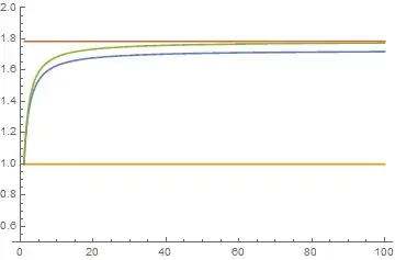
In the above figure,

  • the blue curve corresponds to the numerical values for $g$, i.e., $y(x)=g(x)$,
  • the green curve stands for the upper bound estimate for $g$, i.e., $y(x)=\arctan x+1-\pi/4$, as is mentioned in above,
  • the red line implies the limit value of this green curve, i.e., $y(x)=1+\pi/4$, and
  • the orange line indicates the lower bound of $g$, i.e., $y(x)=1$.

The value of $\alpha$ would be exactly the limit value of the blue curve. You may see that this value is close to, but seemingly not equal to, the limit value of the green curve $1+\pi/4$.

hypernova
  • 6,260
1

Here is a third approach. Introduce a new independent variable $t$ by means of $$x:={1\over 1-t}\qquad(0\leq t<1)\ .$$ Rewriting the given ODE in terms of $t$ leads to the IVP $$\dot y={1\over 1+y^2(1-t)^2}\ ,\qquad y(0)=1\ ,$$ where now $t=1$ doesn't seem to be problematical. Setting up a power series for $t\mapsto y(t)$ and equating coefficients one (that is: Mathematica) obtains $$y(t)=1 + {1\over2}t + {1\over8}t^2 + {1\over12}t^3 + {11\over384} t^4 + {5\over384} t^5 + {1\over3072}t^6 - { 109\over32256} t^7 - {10673\over2\,064\,384} t^8 - {29375\over6\,193\,152} t^9 - {190\,555\over49\,545\,216} t^{10}+\ldots$$ Note that $a_{10}\doteq0.00385$, making it plausible that the series converges also for $t=1$. At any rate the plot of this $y(t)$ looks as expected, and we obtain the numerical value $y(1)=1.73319$, corroborating hypernova's calculations.