The answer depends on your goal. Do you want to (a) Smooth the histogram to get
an estimate of what the population density may look like? (b) Know whether the data are consistent with a particular type of distribution (such as normal)? (That is, possibly to put a "name" to the distribution.) (c) Use the data to estimate the population mean, variance, etc? Feasible goals may depend on how much data you have.
I will briefly explore how to pursue a few of these possible goals.
Data Here are $n = 80$ observations generated from $\mathsf{Norm}(\mu = 100, \sigma = 20)$ and rounded to integers. Examples will be based on them.
I used R statistical software to generate the data. If you used the same seed
I did in R, you could reproduce the data without re-entering it. [Numbers in brackets give the index of the first number on each row.]
set.seed(1212);  x = sort(round(rnorm(100, 100, 20)));  x
 [1]  55  57  62  64  70  72  73  73  73  74  75  79  80  80  81  81  82  83  83  84
[21]  84  85  85  86  87  90  90  90  90  91  92  93  93  93  94  95  95  95  97  97
[41]  97  98  98  98  98 101 101 102 102 104 105 105 105 105 107 108 108 109 109 110
[61] 110 111 111 111 111 112 112 117 118 119 122 124 126 127 133 137 141 142 150 153
Density Estimation.
Of course, you can look at a histogram of the data and try to smooth off the bars, drawing a curve 'by eye'. A modern, mostly objective way to do this is
to use 'kernel density estimation' (KDE). Roughly speaking, KDE patches together many smooth curves to get a resulting estimate of the population density
function that might have produced the data. The process is not entirely
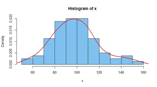
objective because the user can specify the shapes and widths of the curves that are patched together. Here is a density histogram (area of all bars is unity)
with the default version of the KDE in R.
hist(x, prob=T, col="skyblue2")
lines(density(x), type="l", col="red", lwd=2)
Test for normal data. There are several tests to see whether data fit
well to some normal distribution. One of the best of these is the Shapiro-Wilk
test. It gives P-values between $0$ and $1.$ For data sampled at random from
a normal distribution, it rarely gives a P-value less than 0.05. A P-value
greater the 0.05 does not 'prove' the data are normal, but it does indicate
data are consistent with a normal population. Here the P-value is 0.2915.
shapiro.test(x)

        Shapiro-Wilk normality test

data:  x
W = 0.98128, p-value = 0.2915
Estimates of population mean and standard deviation.
For data with as many as $n = 80$ observations that are normal or nearly normal,
one can use Student's t distribution to get a 95% confidence interval for
the population mean $\mu.$
The sample mean and standard deviation of our data are $\bar X = 98.25$ and
$S = 20.33$ These are 'point estimates' of the population
mean $\mu$ and standard deviation $\sigma,$ respectively. [In a real application we will never know the exact values of $\mu$ and $\sigma.$ Because these are
fake simulated data we happen to know that the estimates are pretty good.]
mean(x); sd(x)
## 98.25
## 20.33486
A confidence interval for $\mu$ based on the t distribution is $(93.72,\, 102.78).$
The relevant part of the R output is shown below. It is also possible to get an interval estimate $(17.60,\, 24.09)$ of $\sigma$ using the chi-squared distribution.
t.test(x)

...
data:  x
95 percent confidence interval:
93.7247 102.7753
...
${}$
sqrt(79*var(x)/qchisq(c(.975,.025),70))
## 17.59886 24.08608
Distribution Identification Procedure. Minitab statistical software
has a procedure that compares (nonnegative) data with a large number of
parametric families of distributions to see which are consistent with
the data. In the current version of Minitab, this procedure is in the menu
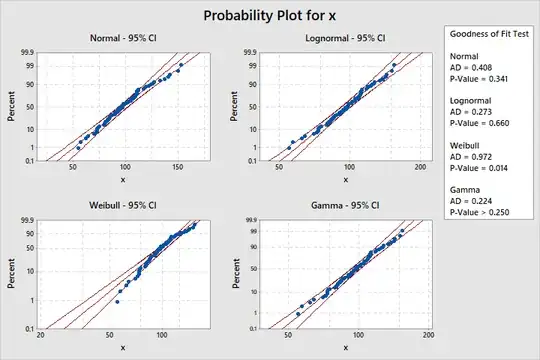
path 'STAT > Quality > Individual distribtion ID'. Here are probability
plots (also called 'quantile-quantile' or 'Q-Q' plots) comparing out data
with normal, lognormal, gamma, and Weibull distributions. All but the
Weibull family might be used to fit our data. (Data that fit should stay
mainly between the colored bands.)
This kind of ambiguity of fit is
common for sample sizes as small as $n = 80.$ In general, it is not
possible to say that a dataset clearly fits any one particular type of distribution.
The maximum likelihood estimates within the families are as follows:
ML Estimates of Distribution Parameters

Distribution  Location     Shape      Scale  Threshold
Normal*       98.25000             20.33486
Lognormal*     4.56620              0.20934
Weibull                  5.06738  106.53068
Gamma                   23.62463    4.15880

* Scale: Adjusted ML estimate
Comments. In your question, you specifically ask about the beta
family of distributions. Ordinarily, the beta family takes values in
$(0,1)$ and would not be suitable to model running times in a 100m race.
(You can read online about a 'generalized beta distribution' that might work.)
Perhaps you meant 'gamma', which might be a very good choice, and is covered
above.
If you have a particular feasible family in mind, then you can check in
a textbook (or on Wikipedia) to see how maximum likelihood estimates of
the distribution parameters are found. For some distributions it is easy
to find estimates, but in some cases special computational methods are
necessary.
Your questions is quite vague. Maybe something discussed here is close to an answer. Maybe something here will help you to refine
your questions so that one of us can give a more satisfactory answer.
But be sure to explain your purpose in wanting to identify the distribution.

