30

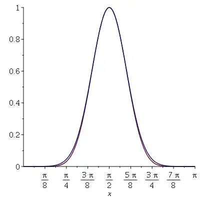
As part of approximating an integral, I have noticed that $\sin^k(x), x\in[0, \pi]$ look almost identical to $\exp\left(-\frac{k}{2}(x-\frac{\pi}{2})^2\right)$ once $k$ is large enough (in practice, the two equations are visually identical for $k\geq 15$). As an example, see this picture of the two functions for $k=10$:

enter image description here

Can anybody explain why these functions practically are identical?

Edit: I should mention that the expression $\exp\left(-\frac{k}{2}(x-\frac{\pi}{2})^2\right)$ is derived by a 2nd order Taylor expansion of $\log\sin^k(x)$ around the mode $x_0 = \frac{\pi}{2}$, i.e. a Laplace approximation.

pipe
  • 105
  • 1
    Have a look at https://math.stackexchange.com/questions/1359813/solving-for-a-in-this-equation-sinaa-b/1492271#1492271 It could be of interest to you. – Claude Leibovici May 23 '17 at 12:38
  • One thing to note is that if $f(x)\approx a(1-b(c-x_0)^2)$ (i.e. $f(x)$ has a local max at $x_0$) then $f(x)^k \approx a^k(1-kb(x-x_0)^2)$. Thus $f(x)^k$ will also have a maximum at $x_0$, and moreover this will be a narrower max. So this is fairly generic. (Try $f(x)=x(1-x)$ to see this in action.) – Semiclassical May 23 '17 at 12:52
  • @ClaudeLeibovici, thanks. That post seems to be concerned with $\sin^x(x)$ whereas I'm interested in $\sin^k(x)$ for some constant $k$. I don't see the immediate connection between these two settings, but perhaps I'm just missing something obvious? – Søren Hauberg May 23 '17 at 13:08
  • @Semiclassical If I approximate $\sin^k(x)$ with a second order polynomial around the mode $x=\frac{\pi}{2}$ then I would get a good approximation of $\sin^k(x)$ nearby the mode. That much I understand. What I don't understand is why $\exp(-\frac{k}{2}(x-\frac{\pi}{2})^2)$ is such a good approximation even at points that are far away from the mode. – Søren Hauberg May 23 '17 at 13:13
  • "All roads lead to the Gaussian"! I know it's not strictly mathematical, but I would maintain there's a great deal of truth in it. Like the way when you have some agglomeration of random variables, each of which has a distribution that might be very far from Gaussian, those individual non-Gaussian-nesses get 'washed-out' as the number of random variables increases, and the result tends towards being Gaussian. It's like the Gaussian is some kind of attractor, or occupies some basin of attraction in the space of functions. – AmbretteOrrisey Dec 02 '18 at 22:19

5 Answers5

37

It's easier to shift $x$ by $\pi/2$ and establish the property for the cosine.

From Taylor and the limit definition of the exponential, for small $x$

$$\cos^kx\approx\left(1-\frac{x^2}2\right)^k=\left(1-\frac{kx^2}{2k}\right)^k\approx e^{-kx^2/2}.$$

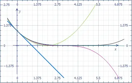
enter image description here

The plot shows good convergence of $(1-t/k)^k$ to $e^{-t}$.

8

This is too long for a comment.

Semiclassical made a very good comment.

Let us use Taylor series around $x=\frac \pi 2$ $$\sin(x)=1-\frac{1}{2} \left(x-\frac{\pi }{2}\right)^2+\frac{1}{24} \left(x-\frac{\pi }{2}\right)^4+O\left(\left(x-\frac{\pi }{2}\right)^6\right)$$ $$\sin^k(x)=1-\frac{1}{2} k \left(x-\frac{\pi }{2}\right)^2+\frac{1}{24} k (3 k-2) \left(x-\frac{\pi }{2}\right)^4+O\left(\left(x-\frac{\pi }{2}\right)^6\right)$$ On the other hand $$e^{-\frac{1}{2} k \left(x-\frac{\pi }{2}\right)^2}=1-\frac{1}{2} k \left(x-\frac{\pi }{2}\right)^2+\frac{1}{8} k^2 \left(x-\frac{\pi }{2}\right)^4+O\left(\left(x-\frac{\pi }{2}\right)^6\right)$$ Computing the difference $$\sin^k(x)-e^{-\frac{1}{2} k \left(x-\frac{\pi }{2}\right)^2}=-\frac{1}{12} k \left(x-\frac{\pi }{2}\right)^4+O\left(\left(x-\frac{\pi }{2}\right)^6\right)$$ AT least, they are very close in the area around the maximum.

5

Another observation too long for a comment:

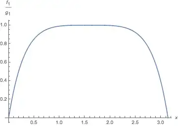
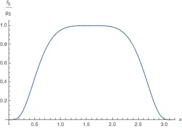
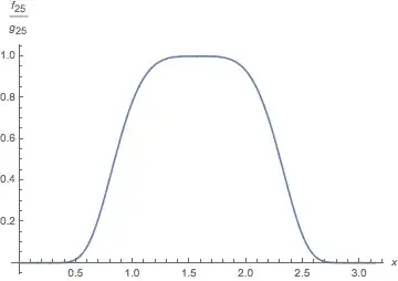
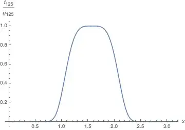
It's not actually that good of an approximation if you look at the ratio of $f_k(x) = \sin^k(x)$ to the value of the $g_k(x) = \exp ( - k (x- \pi/2)^2)$ for various values of $k$. Here are a few plots:

k = 1:

enter image description here

k = 5:

enter image description here

k = 25:

enter image description here

k = 125:

enter image description here

This trend seems to continue as $k$ increases.

  • 1
    That is very interesting! It seems that the regions of low relative difference are the regions where both $f_k$ and $g_k$ are close to zero, right? I ran into this problem when trying to compute an integral of the form $\int_0^{\pi} f(x) \sin^k(x) dx$, where $f$ is a positive function. In this case, I think the regions where $f_k \approx 0$ are of less interest (not sure, though). – Søren Hauberg May 23 '17 at 13:50
  • 1
    @SørenHauberg I think it's actually the opposite: The approximation is good when the graph $f_k/g_k$ is close to $1,$ poor when the graph is close to zero. The "good" part is around the maximum of $f_k$ or $g_k$ and gets narrower as $k$ increases. On the other hand, the Gaussian also gets narrower as $k$ increases, and (I think) faster. It would be interesting to scale the $x$ axis in order to keep the standard deviation of the Gaussian constant, and see whether the "good" part still shrinks or grows. – David K May 23 '17 at 20:04
  • 1
    Being almost blind, I cannot see your plots. However, my wife (she does not know anything about mathematics) told me that they are very explicit. I suppose that they reflect the fact that $$\frac{f_k}{g_k}=1-\frac{1}{12} k \left(x-\frac{\pi }{2}\right)^4-\frac{1}{45} k \left(x-\frac{\pi }{2}\right)^6+O\left(\left(x-\frac{\pi }{2}\right)^7\right)$$ Is this correct ? – Claude Leibovici May 24 '17 at 03:51
  • @ClaudeLeibovici: Yes, basically. As $k$ increases, the leading-order deviation terms (proportional to $(x - \pi/2)^4$ and $(x - \pi/2)^6$) increase in size as well, which means that the ratio is "close to 1" in a smaller and smaller region. – Michael Seifert May 24 '17 at 12:48
3

Yet another observation too long for a comment:

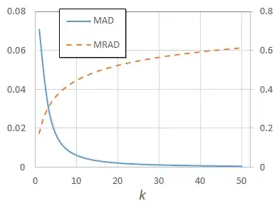
Michael Seifert notes that the quality of match in the relative deviation of the two functions at hand worsens as $k$ is increased. However, the absolute deviation does improve with increasing $k$, as noted by OP.

Plot of MAD and MRAD

Here MAD is the mean absolute deviation between the two functions, while MRAD is the mean relative absolute deviation, calculated at each point with reference to the value of the OP's Gaussian-type function. Both were calculated over the OP's $x\in [0,\pi]$ domain on a grid with spacing $\Delta x=\pi/100$.

So, the "quality of match" of the two functions with increasing k depends entirely on whether the relative or absolute deviation is most relevant to the application at hand.

hBy2Py
  • 347
1

One thing that obscures the point in this exercise is that as $k$ increases, the Gaussian curve $y = \exp\left(-\frac k2(x-\frac\pi2)^2\right)$ develops a very narrow peak in the curve near $x=\frac\pi2$ surrounded by tails that are nearly zero. As long as the values of $\sin^x(x)$ are close enough to $\exp\left(-\frac k2(x-\frac\pi2)^2\right)$ near the very narrow top of the peak, the slope along the sides of the peak ($y$ values between $0.2$ and $0.9$ or other suitable bounds) becomes so steep that you could have a vertical error of several percent and the graphs would still appear very close because of the small horizontal distance to the nearest point on the other curve.

As it turns out, the approximation is really quite good, but it's hard to be sure just by looking at these graphs.

I think we get a better-controlled comparison when we compare all of the approximations to the same Gaussian.

To make things a little simpler, I suggest first shifting the graph left so that it is centered on the line $x=0$ instead of $x=\frac\pi2.$ After this shift, we would be comparing $\cos^x(x)$ with $\exp\left(-\frac k2 x^2\right).$

Next, we expand the graph in the horizontal direction by a factor of $\sqrt k.$ That is, we substitute $\frac x{\sqrt k}$ for $x.$ The Gaussian function then is $\exp\left(-\frac12 x^2\right).$ So we now will be comparing the sequence of sinusoidal functions $h_k(x) = \cos^k\left(\frac{x}{\sqrt k}\right)$ with the Gaussian $f(x) = \exp\left(-\frac12 x^2\right).$

Plotting both $f$ and $h_k$ on the same graph, it is clear that $h_k$ approximates $f$ reasonably well over a wide interval for moderately large values of $k$. (For any particular $k,$ of course, $h_k$ will take the value $1$ at infinitely many values of $x,$ but as $k$ increases the gap between these values of $x$ increases.) Moreover, if we consider the relative error $\frac{h_k}{f} - 1,$ it is visually close to zero for $-\frac12 < x < \frac12$ even for $k=1,$ and the "flat" part of the curve $\frac{h_k}{f} - 1$ gets wider as $k$ increases.

For example, consider this Wofram Alpha graph. It shows that the error of $h_{100}$ relative to $f$ is less than half a percent when $-1.5 < x < 1.5.$

Taking a hint from Semiclassical and Claude Leibovici, let's consider the Taylor series of these functions. The Taylor series of $\exp\left(-\frac12 x^2\right)$ is $$ f(x) = 1 - \frac{x^2}{2} + \frac{x^4}{8} - \frac{x^6}{48} + \mathcal O(x^7). $$

The Taylor series of $\cos^k\left(\frac{x}{\sqrt k}\right)$ is $$ h_k(x) = 1 - \frac{x^2}{2} + \left(\frac18 - \frac{1}{12 k}\right) x^4 - \left(\frac1{48} - \frac1{24k} + \frac1{45k^2}\right) x^6 + \mathcal O(x^7). $$

It's clear that for any $x,$ at least the first two terms of the difference $$ f(x) - h_k(x) = \frac{1}{12 k} x^4 - \left(\frac1{24k} - \frac1{45k^2}\right) x^6 + \mathcal O(x^7) $$ disappear as $k \to\infty$; it seems that the other terms disappear as well.
David K
  • 108,155