First, beta distributions with both shape parameters below 1 are bimodal. The support of a beta distribution is $(0,1),$ and these beta distributions have
probability concentrated near $0$ and $1$.
Second, mixtures of normal distributions can be bimodal, roughly speaking, if the two normal
distributions being mixed have means that are several standard deviations apart.
For example, a 50:50 mixture of $\mathsf{Norm}(\mu=5, \sigma=2)$ and
$\mathsf{Norm}(\mu=10, \sigma=1)$ is noticeably bimodal. (The mixture
distribution is has a density function that is the average of the density
functions of the two distributions being mixed. If the two SDs are equal, you
may want to investigate the exact separation between the means for bimodality.)
I'm not sure what you mean by 'sticking' samples together. Certainly,
if you just concatenate a sample of size 50 from $\mathsf{Unif}(0,1)$ with a
sample of size 50 from $\mathsf{Unif}(2,4),$ you will get a bimodal
histogram with 100 observations, but I personally wouldn't consider that to be random sampling from a bimodal distribution. If you randomly select 100 times from one of two different random samples (each of size 100) at each step, then the result is a random sample from a mixture distribution, which may be bimodal.
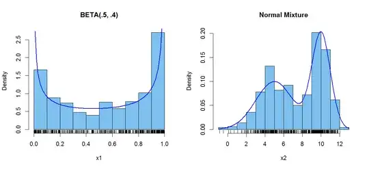
Here is R code to get samples of size $n = 500$ from a beta distribution and a bimodal normal
mixture distribution, along with histograms of the two datasets, with the
bivariate densities superimposed.
Notes: (1) I use $n = 500$ instead of $n = 100$ just for
illustration, so you can see that the histograms are close to matching the
bimodal densities. (2) This is very simplistic R code, which you should adapt
to whatever software you're using and to your degree of sophistication using it.
(3) I don't know if you are allowed to use pre-programed functions, such as
rbeta and rnorm, that sample from specific distributions, or whether
you are supposed to use the inverse-CDF method with uniform observations.
 set.seed(1234)                            # include seed for same samples
 n = 500;  x1 = rbeta(n, .5, .4)
 y1 = rnorm(n, 5, 2);  y2 = rnorm(n, 10, 1)
 w = rbinom(n, 1, .5)                      # 50:50 random choice
 x2 = w*y1 + (1-w)*y2                      # normal mixture
 par(mfrow=c(1,2))                         # two panels per plot
   hist(x1, prob=T, col="skyblue2", main="BETA(.5, .4)");  rug(x1)
     curve(dbeta(x, .5, .4), lwd=2, col="blue", add=T)
   hist(x2, prob=T, col="skyblue2", main="Normal Mixture"); rug(x2)
     curve(.5*dnorm(x,5,2)+.5*dnorm(x,10,1), lwd=2, col="blue", add=T)
 par(mfrow=c(1,1))                         # return to default single panel
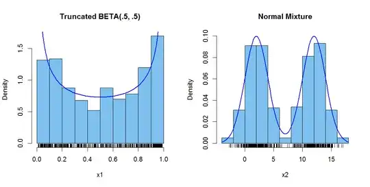
Addendum: (After Comments) It seems you define a bimodal PDF to mean two
achieved maximums of equal height. Slight modifications in the code are
as follows, with additional comments at the changes:
set.seed(1235)
n = 2000;  u1 = rbeta(n, .5, .5)           # 2000 wasteful, but simple
cond = u1 > .01 & u1 < .99
v1 = u1[cond];  x1 = v1[1:500]             # truncate and use 500
n = 500; y1 = rnorm(n, 2, 2);  y2 = rnorm(n, 12, 2)  # same SD
w = rbinom(n, 1, .5)
x2 = w*y1 + (1-w)*y2
par(mfrow=c(1,2))
  hist(x1, prob=T, col="skyblue2", main="Truncated BETA(.5, .5)");  rug(x1)
    k = diff(pbeta(c(.01,.99),.5,.5))      # adj for truncation
    curve((1/k)*dbeta(x, .5, .5),.01,.99, lwd=2, col="blue", add=T)
  hist(x2, prob=T, col="skyblue2",ylim=c(0,.1), main="Normal Mixture"); rug(x2)
    curve(.5*dnorm(x,2,2)+.5*dnorm(x,12,2), lwd=2, col="blue", add=T)
par(mfrow=c(1,1))


rbeta. CDF of arcsine dist'n easy to invert. And then there is Feller's Arcsine Law. Sometimes discussions of bimodal distributions give only symmetrical examples, and I wanted to illustrate asymmetrical ones. – BruceET Feb 18 '17 at 16:35