A few examples include:
- The polar set of a singleton $\{x\}$ is a halfspace with support hyperplane orthogonal to $x$. If $\|x\|=1$ then the halfspace touches $x$, otherwise its below $x$ iff $\|x\|>1$:
$\hspace{40pt}$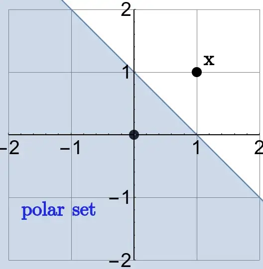
The polar set of a unit disk is the disk itself.
See this question for the polar set of $\{(x,y)\in\mathbb R^2: x^2+y^4\le1\}$.
Consider the polytope with the four vertices $(\pm 1,\pm1)$ (a square centred at the origin). Then its polar set is a rotated square with vertices $(0,\pm1),(\pm1,0)$:
$\hspace{40pt}$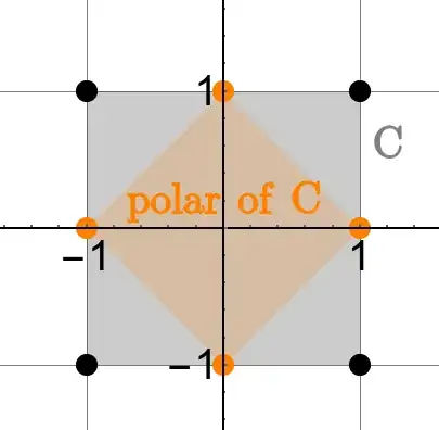
You can find more examples in these lecture notes by Jonathan Kelner (Link to pdf).
If you have access to Mathematica, I made a simple snippet to explore how the polar sets of finite numbers of points look like. Just click anywhere to add points and see the corresponding polar set:
$\hspace{40pt}$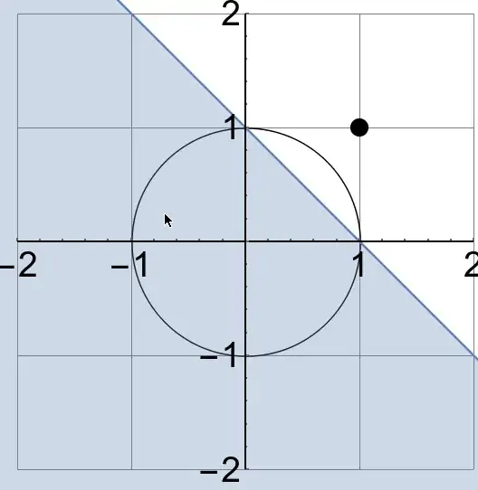
Here's the code to generate this visualisation:
DynamicModule[{pts={{1,1}}},
    EventHandler[
        Dynamic@Show[
            Graphics[{
                PointSize@0.04,Dynamic@Point@pts,
                Circle[]
            },
                Axes->True,AxesOrigin->{0,0},Frame->False,PlotRange->ConstantArray[{-2,2},2],
                GridLines->Automatic,AxesStyle->Directive[Large,Black]
            ],
            RegionPlot[
                And@@(Dot[#,{x,y}]<=1&/@pts),
                {x,-4,4},{y,-4,4},PlotPoints->50
            ]
        ],
        {"MouseClicked":>(AppendTo[pts,MousePosition["Graphics"]])}
    ]
]
See source of this answer for the MMA code used to generate the figures.