Sigmoid function with fixed bounds and variable steepness [partially solved]

Question

(see edits below with attempts made in the meanwhile after posting the question)

Problem

I need to modify a sigmoid function for an AI application, but cannot figure out the correct math. Given a variable $x \in [0,1]$, a function $f(x)$ should satisfy the following requirements (pardon the math-noobiness of my expression):
a) the values of $f(x)$ should be costrained to $[0,1]$
b) when $x=0$ then $f(x)=0$, and when $x=1$ then $f(x)=1$
c) $f(x)$ should follow a sigmoid or "S-curve" shape within these bounds, with some variable changing the "steepness" of the curve.

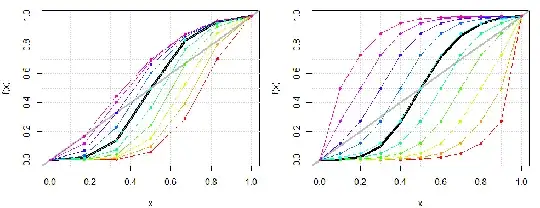
I used a different function earlier, corresponding to (0), illustrated below on the left:

(0) $f(x) = x^{(z+0.5)^{-b}}$ , where $b=2$ with $z \in [0,1]$ controlling the curve

What is a function that would satisfy these requirements, i.e. do the same thing as equation (0) but with an S-curve$?_{(I\hspace{1mm} hope\hspace{1mm} this\hspace{1mm} makes\hspace{1mm} at\hspace{1mm} least\hspace{1mm} some \hspace{1mm}mathematical\hspace{1mm} sense...)}$

---

Attempt 1

I tried to accomplish something similar with a logistic function (by varying the $x_0$ value; cf. equation (1) and the right side plot above)

(1) $f(x) = \dfrac{1}{1 + e^{-b(x-(1-x_0))}}$ , where $b=10$, $x_0 \in [0,1]$

...so that $x_0 = 0.5$ yields some central or average curve (like the linear growth line on the leftmost plot), and values around it rise or lower the steepness. Shortcoming: the "ends" of the curve where $x=\{0,1\}$ won't reach the required values of 0 and 1 respectively. I don't want to force it arbitrarily with an if-else, it should come naturally from the properties of an equation (and as such form nice curves).

Attempt 2

This sort of does the trick, now the ends smootly reach 0 and 1 for all values of $x_0$:

(2) $f(x) = \Bigg(\bigg( \dfrac{1}{1 + e^{-b(x-(1-x_0))}}\bigg)x\Bigg)^{1-x} $

Only problem, the effect is not "symmetrical", when comparing high and low values. Observe the values for $f(x)$ with $x_0 = [0,1]$; $b=10$ (left side plot below). The curve steepness varies more among lower $x_0$ values (yellow,red) than amoing higher values (pink); also, changing $x_0$ also has noticably more effect in lower values of $x$ than its higher values.

Attempt 3

Ok maybe if-elsing the hell out of those extreme values is not such a bad idea.

(3) $f(x) = \Bigg(\bigg( \dfrac{1}{1 + e^{-b(x-(1-x_0))}}\bigg)g(x)\Bigg)^{1-h(x)} $

where $g(x) = \left\{\begin{array}{ll}1 & x>0\\0 & otherwise\end{array}\right.$ and $h(x) = \left\{\begin{array}{ll}1 & x==0\\0 & otherwise\end{array}\right.$

The right side plot above illustrates the result: the ends are still nicely 0 and 1, and now the curves above and below $x_0=0.5$ are symmetrical, but there are noticable "jumps" on $x=0.1$ and $x=0.9$ if $x_0$ is in its either extremes. Still not good.

---

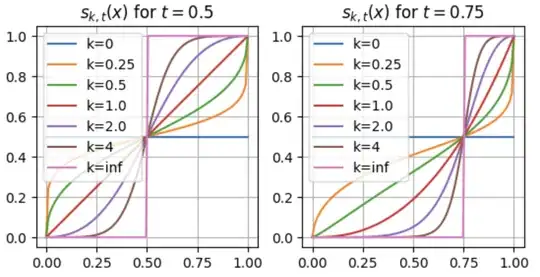
So far all my attempts are all so-so, each lacking in some respect. A better solution would thus still be very welcome.

Answer 1

I was just working on finding a similar function. In case anyone else lands here in the future, here is a sigmoidal function which satisfies:

$$f(0)=0$$ $$f(1)=1$$

and has a single parameter, $k$, controlling steepness:

$$f(x) = 1-\frac{1}{1+(\frac{1}{x}-1)^{-k}} $$

Note that, by symmetry, these will also always be true: $f(1/2)=1/2$, and $\int_0^1 f(x)dx = 1/2$.

Method: Since $\frac{1}{1+e^x}$ is a bijection from $\mathbb{R} \to [0,1]$; we can invert it to get a function mapping $[0,1] \to \mathbb{R}$, which is $h(x) = \ln(\frac{1}{x}-1)$. Then we can put $h$ into a standard (increasing) sigmoid which maps the reals back to $[0,1]$. The form of the sigmoid is:

$$ g(y) = 1-\frac{1}{1+e^{-ky}}$$

$f(x)$ is what you get when you simplify $g(h(x))$. Note that this $f$ is defined outside $x \in [0,1]$ and it does not asymptote out to 0 or 1, but it does achieve the desired behavior within that interval.

One additional note, in the special case where $k=1$, this function reduces to $f(x)=x$.

Answer 2

To expand on Ron's answer, we can generalize to allow our "bounded sigmoid" to cross the $y=0.5$ line at a chosen position of x, using the solution to this related post, giving us a "generalized bounded sigmoid" function $s_{k,t}(x)$ where $k\in[0, \infty)$ controls the steepness and $t\in(0, 1)$ controls the threshold. This function has the following properties:

• $s_{k,t}(0)=0; \forall k, t$ (Starts in bottom left)
• $s_{k,t}(1)=1; \forall k, t$ (Ends in top right)
• $s'_{k, t}(x) > 0; \forall k >0$ (Stricty monotonic in x)
• $s_{k,t}(t)=\frac12; \forall k$ (Crosses $s_{k,t}(x)=\frac12$ at x=t)
• $s'_{k, t}(t) \propto k$ (The slope at the 'threshold' point is proportional to k, with equality for $t=\frac12$)

The Equation

$$\begin{align} f_k(x) &= \frac{1}{1+\big(\frac1x-1 \big)^{k}} \text{... Ron's answer after Tim's simplification}\\ g_t(x) &= x^\frac{-\log2}{\log t} \text{... A monotonic function passing through $[(0, 0), (t, 0.5), (1, 1)$]} \\ s_{k,t}(x) &= f_k(g_t(x)) \text{... Compose the two solutions} \\ &= \frac{1}{1+\left(x^{\frac{\log 2}{\log t}}-1 \right)^k} \end{align}$$

This gives a nice, smooth, bounded-sigmoid function where you can adjust both threshold-crossing-slope $k$ and "soft-threshold" $t$.

See Colab Notebook.

Answer 3

Look for this substitution (kx-x)/(2kx-k-1) x from 0 to 1 k from -1 to 1 Then you can scale the argument if you will need

https://dinodini.wordpress.com/2010/04/05/normalized-tunable-sigmoid-functions/ http://www.wolframalpha.com/input/?i=(kx-x)%2F(2kx-k-1)+x+from+0+to+1+k+from+-1+to+1