There are many different kinds of bootstrap CIs, even for the basic case of finding a CI for the population mean $\mu$ of a sample based on a sample from the population. Here is a concrete example of one of them along with a brief rationale for the bootstrap method illustrated.
Here is a sample of size $n=20$ that pretty clearly does not come from a normal population. It decisively fails the Shapiro-Wilk normality test, and it has three far outliers as shown in the boxplot.
 x = c( 29,  30,  53,  75,  89,  34,  21,  12,  58,  84,
        92, 117, 115, 119, 109, 115, 134, 253, 289, 287)
 shapiro.test(x)
Shapiro-Wilk normality test


data:  x
 W = 0.8347, p-value = 0.002983

A bootstrap CI makes no distributional assumption about the population. All that is 'known' is that the population is capable
of producing the $n$ observations in the population at hand.
In an ideal situation, we would know something about the variability of the data around $\mu.$ Specifically, we might know the distribution of $V = \bar X - \mu,$ from which we could find a 95% CI for $\mu$ by traditional means. In that case, we could find $L$ and $U$ cutting 2.5% from the upper and lower tails, respectively, of the distribution of $V$, and we could write
$$P(L \le V = \bar X - \mu \le U) = P(\bar X - U \le \mu \le \bar X - L) = .95.$$
so that a 95% CI for $\mu$ would be $(\bar X - U, \bar X - L).$
However, we do not know $U$ and $L$.
Entering the 'bootstrap world', we use resampling, to find
approximate values $U$ and $L$ as follows:
(1) Take $X_i, \dots, X_n$ to be the 'bootstrap population'.
(2) The mean of this population is $\mu^* = \bar X.$
(3) Simulate many values $V^*$ of $V$ by resampling: Repeatedly
select a sample of size $n$ with replacement from $X_1, \dots, X_n$.
For each resample, find the mean $\bar X^*$ and then $V^* = \bar X^* - \mu^*.$ Below we use $B = 100,000$ resamples of size $n = 20.$
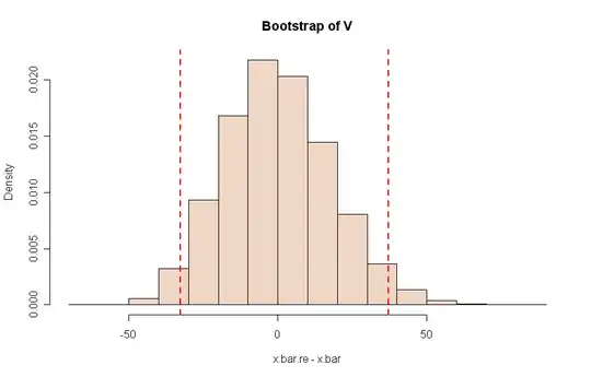
(4) Find cutoff points $L^*$ and $U^*$ of the resample distribution $V^*.$
Then, back in the 'real' world use these proxy cutoff values to make
the bootstrap CI $(\bar X - U^*, \bar X - L^*)$ for $\mu.$
Notice that $\bar X$ plays two roles here: first, as the population
mean $\mu^*$ of the 'population' from which we resample; second, as
itself (the mean of the original sample).
In R, this procedure can be programmed as follows, where .re
(for resample) represents the stars $*$ in the notation above.
 x = c( 29,  30,  53,  75,  89,  34,  21,  12,  58,  84,
        92, 117, 115, 119, 109, 115, 134, 253, 289, 287)
 x.bar = mean(x); n = length(x)
 B = 100000;  x.bar.re = numeric(B)
 for (i in 1:B) {
    x.bar.re[i] = mean(sample(x, n, repl=T))  }
 L.re = quantile(x.bar.re - x.bar, .025)
 U.re = quantile(x.bar.re - x.bar, .975)
 c(x.bar - U.re, x.bar - L.re)
 ##  97.5%   2.5%
 ##  68.25 138.30
Thus a 95% CI for $\mu$ is $(68.25, 138.30).$ Because this is
a random process, the result will be slightly different on each
run of the program. Differences are slight for $B$ as large
as $B = 100,000,$ as here. Two subsequent runs gave $(68.7, 138.3)$
and $(68.35, 138.45).$
A histogram of the resample distribution $V^*$ from one run of this program is shown below.
Notes: (a) A naive, and often misleading, approach is sometimes used.
Simply, find $\bar X^*$ on each resample, and cut 2.5% from
each tail of the resulting distribution of these $\bar X^*$s. This
approach is sometimes used for symmetrical data, but would not
work well for the current skewed sample.
(b) A 95% t interval for the population mean $\mu$ is $(67.17, 144.33),$
a result that is in some doubt because of the rather extremely
nonnormal data. (c) A 95% CI for the population median $\eta$
based on a Wilcoxon procedure is $(64.5, 141.5).$ But the population seems skewed so that we may have $\mu > \eta.$

