The "find my car" problem: proper interpretation and solution?

Question

This has been asked at least twice here, but both questions have accepted answers which are wrong. I don't really know any good way to draw attention to the question besides asking again and being a bit more careful about not accepting incorrect or incomplete answers, so here goes.

Say I am standing at the origin of the real line, and I know my car is somewhere on the real line. The PDF is a normal curve. I want to search for it optimally walking at a fixed pace. The problem is, if I look right and it really was left, I'm going to, at some point, have to back track to find it. So let's see if we can model this more formally.

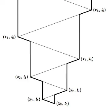
The set of times is $\mathbb R^+$, so I want a continuous, rigid (so that one "second" becomes one "unit") transformation $f$ with $f(0) = 0$.

A few definitions:

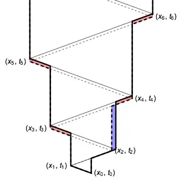
• Let $S_f(t)$ (success of $f$) be the probability that the car is found by time $t$. It equals $\int_{\min f}^{\max f}N(\mu, \sigma)(x)dx$, Where the $\min$ and $\max$ are taken on $[0,t]$. So it's the amount of area under the normal curve that is covered.
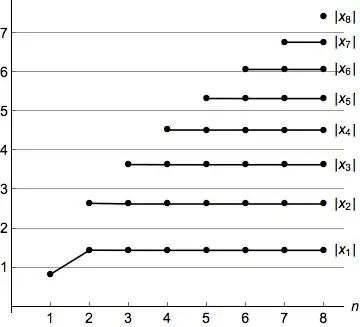
• For a fixed $x \in \mathbb R$ where the car might be, let $T_f(x)$ be the amount of time it takes to find $c$. This is $\min \{t: f(t) = c\}$.
• Define $P_f(p)$ for $0 < p < 1$ to be the amount of time it will take to have found the car with probability $p$. That is, $P_f(p) := \min \{t \in \mathbb R^+ : S_f(t) \geq p \}$.

I think there are a few valid interpretations of this problem:

1. For a fixed amount of time $t$, find $f$ to maximize $S_f$. I don't think $f$ is independent of $t$, because backtracking takes time, and taking a function that backtracks and telling it, "you don't have time to backtrack all the way back," would tell it not to backtrack at all.
2. Find an $f$ whose expected value of $T_f$ where $x$ is normally distributed is smallest. I think this is closest to the real world problem.
3. For a fixed probability $p$, find $f$ such that $P_f(p)$, which returns an amount of time, is minimal.
4. Let's put these together. Say you're willing to abort once you have reached a $p$ chance of finding the car. This models reality in the Bayesian sense that once I should have found my car with probability $99.99\%$ by now, then maybe my model needs to be revised and I should look on another street. Consider $J_f(x) := \min(T_f(x), P_f(p))$. Now find $f$ such that the expected value of $J_f$ is smallest over normally distributed $x$.

So the first question is whether I interpreted this question correctly. The second is how to solve any of them.

Answer 1

Any valid search scheme is characterized by an increasing sequence of time intervals $\tau_1<\tau_2<\tau_3<\cdots$ such that for time $\tau_1$ you walk left, then for time $\tau_2$ you walk right, then for time $\tau_3$ you walk left again, and so on. Then your turning points are $$\begin{align} t_1&=\tau_1 & x_1&=-\tau_1 \\ t_2&=\tau_1+\tau_2 & x_2&=-\tau_1+\tau_2\\ t_3&=\tau_1+\tau_2+\tau_3 & x_3&=-\tau_1+\tau_2-\tau_3\\ &\vdots & &\vdots \\ t_n&=\sum_{i=1}^n\tau_i & x_n&=\sum_{i=1}^n(-1)^nt_i \end{align}$$ and we have $$f(t)=x_n+(-1)^{n+1}(t-t_n)\qquad\text{when $t_n\le t\le t_{n+1}$}.$$ Conversely, the first time the point at location $x$ is passed is $$g(x)=t_n+(-1)^{n+1}(x-x_n)\qquad\text{when $x_n\le x\le x_{n+1}$ or $x_n\ge x\ge x_{n+1}$}.$$

---

Let $\underline f(t)=\min_{s\le t}f(s)$ and $\overline f(t)=\max_{s\le t}f(s)$. To maximize $S_f(t)$ for a fixed $t$, it only makes sense to turn around at most once, because any $[\underline f(t),\overline f(t)]$ achieved by turning around multiple times can be achieved in less time by turning around only once. So we may take $\tau_1\le t/2$ (because turning around buys you nothing if $\tau_1>t/2$), and $\tau_{n>1}=\infty$. Then we have $\underline f(t)=-\tau_1$ and $\overline f(t)=t-2\tau_1$, and the task is simply to maximize the probability mass lying in the interval $[-\tau_1,t-2\tau_1]$. For the standard normal distribution, this gives $$S_f(t) = \frac12\operatorname{erf}\left(\frac{\tau_1}{\sqrt2}\right)+\frac12\operatorname{erf}\left(\frac{t-2\tau_1}{\sqrt2}\right)$$ which is maximized when $$\tau_1=\max\left(\frac23t - \frac13\sqrt{t^2+6 \log 2},0\right).$$ Asymptotically, as $t\to\infty$ we get $\tau_1\to t/3$: you should walk in one direction for time $t/3$, then turn around and walk the other way for the rest of the time, so that you cover a symmetrical range. On the other hand, for $t\le\sqrt{2\log 2}$ we have $\tau_1=0$: turning around is not worth the wasted time.

---

Come to think of it, this should also solve question (3), because a solution that maximizes $p$ subject to $t\le t_\max$ also minimizes $t$ subject to $p\ge p^*$, where $p^*$ is the optimum value of the former problem. So you just have to substitute the optimum $\tau_1$ into the expression for $S_f(t)$ to get $S^*(t)$, the highest possible probability of finding the car within time $t$. And then solve $S^*(t)=p$. It doesn't seem to yield an elementary solution, though.

---

Question (2) is a fair bit trickier. Here is a space-time diagram of the situation, with $x$ on the horizontal axis and $t$ on the vertical:

The thin line is $x=f(t)$, and the thick line is $t=g(x)$. We seek to minimize $T_f = \mathbb E[g]$, the expected value of the vertical coordinate of $g$ when the horizontal coordinate is normally distributed. I will not attempt to write down an explicit expression for this quantity. Instead, let us consider its variations under infinitesimal changes of $\tau_n$. At the optimum, any such variation should be zero.

Suppose you increase both $\tau_n$ and $\tau_{n+1}$ by the same amount $\delta t$. For a small $\delta t$-length interval of points near $x_n$, this decreases $g(x)$ from about $t_n+2\tau_{n+1}$ to about $t_n$. However, for all the points visited afterwards, $g(x)$ increases by $2\delta t$. These are shown in blue and red below for $n=2$.

Let $\phi(x)$ denote the probability density at $x$, and $\Phi(a,b)$ the probability mass lying between $a$ and $b$. The probability of the blue region is $\phi(x_n)\delta t$, while that of the red is $1 - \Phi(x_{n-1}, x_n)$. Therefore, the change in $\mathbb E[g]$ is $$\phi(x_n)\delta t\cdot(-2\tau_{n+1}) + \big(1-\Phi(x_{n-1},x_n)\big)\cdot2\delta t.$$ Looking at the diagram again, what we have just computed is $\delta t$ times the partial derivative of $\mathbb E[g]$ with respect to $x_n$, holding the rest of the $x_m$'s constant. At the optimum all the first derivatives should be zero, so $$\phi(x_n)\tau_{n+1} = 1 - \Phi(x_{n-1},x_n)$$ for all $n\ge 1$. It appears that the natural parametrization of the problem is in terms of $x_n$, so we substitute $\tau_{n+1}=|x_{n+1}-x_n|$ and get a nice sequence of equations each involving only three variables: $$\begin{align} |x_2-x_1|\phi(x_1) &= 1 - \Phi(x_0,x_1), \\ |x_3-x_2|\phi(x_2) &= 1 - \Phi(x_1,x_2), \\ |x_4-x_3|\phi(x_3) &= 1 - \Phi(x_2,x_3), \\ &\vdots \end{align}$$

Now all we have to do is solve this infinite system of nonlinear equations. But I don't know how to do that.

---

Well, here's an idea: take the first $n$ equations, eliminate $x_{n+1}$ by assuming $|x_{n+1}|-|x_n|=|x_n|-|x_{n-1}|$, and solve the system numerically.

Seems to work pretty well. For $n=8$, we get $$\begin{align} x_1&=-1.44085,&x_2&=2.62758,&x_3&=-3.6322,&x_4&=4.52034,\\ x_5&=-5.32668,&x_6&=6.07158,&x_7&=-6.76811,&x_8&=7.42555. \end{align}$$

I'm not sure this is really a rigorous technique, and I certainly haven't proved convergence or anything like that. But this is good enough for me.