Can a linear regression model without polynomial features overfit?

Question

I've read in some articles on the internet that linear regression can overfit. However is that possible when we are not using polynomial features? We are just plotting a line trough the data points when we have one feature or a plane when we have two features.

Answer 1

It sure can!

Throw in a bunch of predictors that have minimal or no predictive ability, and you’ll get parameter estimates that make those work. However, when you try it out of sample, your predictions will be awful.

set.seed(2020)
Define sample size

N <- 1000
Define number of parameters

p <- 750
Simulate data

X <- matrix(rnorm(N*p), N, p)
Define the parameter vector to be 1, 0, 0, ..., 0, 0

B <- rep(0, p)#c(1, rep(0, p-1))
Simulate the error term

epsilon <- rnorm(N, 0, 10)
Define the response variable as XB + epsilon
y <- X %*% B + epsilon
Fit to 80% of the data

L <- lm(y[1:800]~., data=data.frame(X[1:800,]))
Predict on the remaining 20%

preds <- predict.lm(L, data.frame(X[801:1000, ]))
Show the tiny in-sample MSE and the gigantic out-of-sample MSE

sum((predict(L) - y[1:800])^2)/800
sum((preds - y[801:1000,])^2)/200

I get an in-sample MSE of $7.410227$ and an out-of-sample MSE of $1912.764$.

It is possible to simulate this hundreds of times to show that this wasn't just a fluke.

set.seed(2020)
Define sample size

N <- 1000
Define number of parameters

p <- 750
Define number of simulations to do

R <- 250
Simulate data

X <- matrix(rnorm(N*p), N, p)
Define the parameter vector to be 1, 0, 0, ..., 0, 0

B <- c(1, rep(0, p-1))
in_sample <- out_of_sample <- rep(NA, R)
for (i in 1:R){
if (i %% 50 == 0){print(paste(i/R*100, "% done"))}
Simulate the error term

epsilon <- rnorm(N, 0, 10)
Define the response variable as XB + epsilon

y <- X %*% B + epsilon
Fit to 80% of the data

L <- lm(y[1:800]~., data=data.frame(X[1:800,]))
Predict on the remaining 20%

preds <- predict.lm(L, data.frame(X[801:1000, ]))
Calculate the tiny in-sample MSE and the gigantic out-of-sample MSE

in_sample[i] <- sum((predict(L) - y[1:800])^2)/800
  out_of_sample[i] <- sum((preds - y[801:1000,])^2)/200
}
Summarize results

boxplot(in_sample, out_of_sample, names=c("in-sample", "out-of-sample"), main="MSE")
summary(in_sample)
summary(out_of_sample)
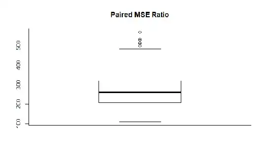
summary(out_of_sample/in_sample)

The model has overfit badly every time.

In-sample MSE summary
   Min. 1st Qu.  Median    Mean 3rd Qu.    Max. 
  3.039   5.184   6.069   6.081   7.029   9.800 

Out-of-sample MSE summary
   Min. 1st Qu.  Median    Mean 3rd Qu.    Max. 
  947.8  1291.6  1511.6  1567.0  1790.0  3161.6 

Paired Ratio Summary (always (!) much larget than 1)
   Min. 1st Qu.  Median    Mean 3rd Qu.    Max. 
  109.8   207.9   260.2   270.3   319.6   566.9 

Answer 2

Ordinary Least Squares (OLS) is quite robust and under Gauss-Markov assumptions, it is a best linear unbiased estimator (BLU). So there is no overfitting as understood to be a problem, e.g. with neural nets. If you want to say so, there is just „fitting“.

When you apply variations of OLS, including adding polynomials or applying additive models, there will of course be good and bad models.

With OLS you need to make sure to meet the basic assumptions since OLS can go wrong in case you violate important assumptions. However, many applications of OLS, e.g. causal models in econometrics, do not know overfitting as a problem per se. Models are often „tuned“ by adding/removing variables and checking back on AIC, BIC or adjusted R-square.

Also note that OLS usually is not the best approach for predictive modeling. While OLS is rather robust, things like neural nets or boosting are often able to produce better predictions (smaller error) than OLS.

Edit: Of course you need to make sure that you estimate a meaningful model. This is why you should look at BIC, AIC, adjusted R-square when you choose a model (which variables to include). Models which are „too large“ can be a problem as well as models which are „to small“ (omitted variable bias). However, in my view this is not a problem of overfitting but a problem of model choice.