How to estimate the variance of regressors in scikit-learn?

Question

Every classifier in scikit-learn has a method predict_proba(x) that predicts class probabilities for x. How to do the same thing for regressors?

The only regressor for which I know how to estimate the variance of the predictions is Gaussian process regression, for which I can do the following:

y_pred, sigma = gp.predict(x, return_std=True)

In one dimension, I can even plot, how confident the Gaussian process regressor is about its prediction of different data points

How to estimate the variance of predictions for other regressors? For example, for kernel ridge regressor, multi-layer perceptron, ensemble regressors?

Answer 1

I believe it is the probabilistic nature of a model that allows you to get the variance of predictions, or more generally defined as the uncertainty of predictions, like the Gaussian process you mentioned. This is not simply avaialble in standard regressors.

I think you should be looking at Probabilistic regressors like BayesianRidge if you would like to estimate the uncertainty of your model. An implementation is also avaialble in scikit-learn, also this nice python package based on PyMC3 or directly via PyMC3 itself for instance. In the latter there are examples like for Bayesian regression in Jupyter Notebook with a good explanation.

In principle, Bayesian Models do not return a a single estimate for the model parameters, but a distribution that make it possible to make inferences about new observations as well as to examine our uncertainty in the model. You may find this post useful.

Note: Adding a normal prior on the weights as it is done in Bayesian regression, one turn the Least-Squares problem to regularized L2 regression under the hood as well (see the full math. derivation here).

Updated Answer: I totally forgot the classical yet simple and powerful Bootstrap Sampling method to calculate confidence intervals for machine learning algorithms. A textbook definition says:

Bootstrapping is a nonparametric approach to statistical inference that substitutes computation for more traditional distributional assumptions and asymptotic results. A number of advantages:

• The bootstrap is quite general, although there are some cases in which it fails.
• Because it does not require distributional assumptions (such as normally distributed errors), the bootstrap can provide more accurate inferences when the data are not well behaved or when the sample size is small.
• It is possible to apply the bootstrap to statistics with sampling distributions that are difficult to derive, even asymptotically.
• It is relatively simple to apply the bootstrap to complex data-collection plans (such as stratified and clustered samples).

Reference: Fox, John. Applied regression analysis and generalized linear models. Sage Publications, 2015.

Please note you do not need a model with probabilistic nature. See this post, or this answer or this one.

Answer 2

You are most likely looking for prediction intervals? You don't need any fancy models to get those, standard linear regression can provide prediction intervals.

https://en.wikipedia.org/wiki/Prediction_interval

A detailed explanation of how to use those are in this fantastic book on statistical learning:

https://www.stat.berkeley.edu/users/rabbee/s154/ISLR_First_Printing.pdf

I made use of these in my masters thesis. They gave good estimates with linear regression for prediction patient appointment duration times.

https://aaltodoc.aalto.fi/items/4cd8dc4a-4a53-44b8-a542-ad7301828126

Answer 3

I have an idea but I am not sure if it is correct. Please feel free to express whatever opinion or emotions you might have about the following solution.

Classification and regression tasks are very similar. If done, for example, via neural networks, then a network for regression will differ from the corresponding network for classification only in activation function of the output neuron and the loss function.

The idea is to bin the target variable for the regression task, make a classification on the binned labels, and then use predict_proba to get the probability of the predicted values to be in a certain interval.

The prediction probability for the initial regression task can be estimated based on the results of predict_proba for the corresponding classification.

This is how it can be done for the same toy problem as shown on the picture in the question. The task is to learn a 1-D gaussian function

def gaussian(x, mu, sig):
    return np.exp(-np.square((x-mu)/sig)/2)

given some training data.

I build the following neural network in Keras:

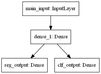
The network is trained simultaneously for both classification and regression. It splits only in the last layer. The input is one-dimensional. The hidden layer has 10 neurons. The output layer for regression is one neuron with the linear activation. The output layer for classification has several softmax neurons. Their amount depends on how many bins are filled with target variables.

In this toy example, I have 6 training data points:

# training data
x_train = np.atleast_2d([3.2487, -1.2235, -10.0, 10.0, -5.7789, 6.6834]).T
y_train = gaussian(x_train, mu, sig)

I divide the whole range were the target variable changes (0 to 1) into 10 bins. Each bin is 0.1 wide. The amount of bins can be thought of as a hyper-parameter. The more bins the closer the classification problem to the corresponding regression problem. But too many bins is probably not good.

# Binning the target variable
hist, bin_edges = np.histogram(y_train, bins=np.linspace(0, 1, 11))
y_c = np.digitize(y_train, bin_edges)
n_classes = len(np.unique(y_c))

# Binarize targets for classification
lb = LabelBinarizer()
y_b = lb.fit_transform(y_c)

The training data fall into three bins. You can see in the picture why. The four points far on each side (two on the left side, and two on the right side) are all in one bin, and each of the remaining points in the middle is in a separate bin. The remaining seven bins are empty. So, the output layer for the classification task has 3 softmax neurons. I use 1-hot encoding for the labels.

This is the network:

# NNet with one input and two outputs: one for reg, another for clf
main_input = Input(shape=(1,), dtype='float32', name='main_input')
hidden = Dense(10, input_dim=1, activation='tanh')(main_input)
reg_output = Dense(1, activation='linear', name='reg_output')(hidden)
clf_output = Dense(n_classes, activation='softmax', name='clf_output')(hidden)
model = Model(inputs=[main_input], outputs=[reg_output, clf_output])

Different loss functions are used for classification and regression. I also assign different loss weights which can be thought of as another hyper-parameter.

model.compile(optimizer='adam',
              loss={'reg_output': 'mse', 'clf_output': 'categorical_crossentropy'},
              loss_weights={'reg_output': 1., 'clf_output': 0.2})

Training:

model.fit({'main_input': x_train},
          {'reg_output': y_train, 'clf_output': y_b},
          epochs=1000, verbose=0)

Running model.predict gives prediction for the regression and prediction probabilities for classification.

# Prediction for both classification and regression 
y_pred, pred_proba_c = model.predict({'main_input': x})

Each row of the array pred_proba_c contains probabilities of putting a test point to one of three classes. I estimate a regression's analogue of predict_proba by taking the maximum of these three probabilities.

# This is a regression's analogue of predict_proba 
r_pred_proba = np.max(pred_proba_c, axis=1)

This is the result. The prediction probability is shown in the bottom half of the picture.

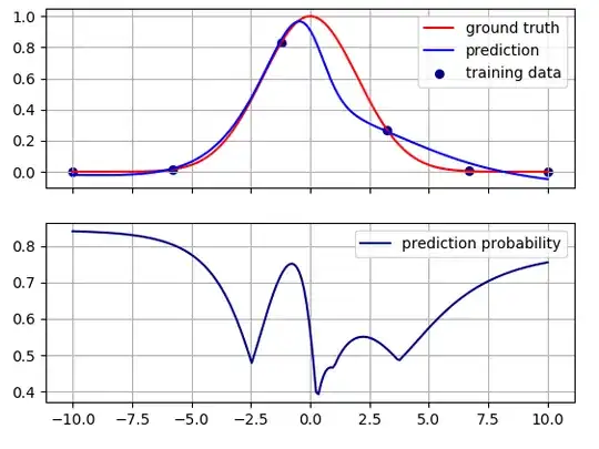
Intuitively, the probability is high where there are training data, and it decreases in the regions between the training data. The model becomes less sure about its predictions far from the training data.

The maxima of the prediction probability are not exactly at the training points. This might be because there is no exact correspondence between the underlying classification and regression problems. They are related but they are not the same, and the relationship between them depends on the values of the hyper-parameters, and the learning algorithm. For example, if I change the loss weights,

model.compile(optimizer='adam',
              loss={'reg_output': 'mse', 'clf_output': 'categorical_crossentropy'},
              loss_weights={'reg_output': 1., 'clf_output': 1})

I get the following picture:

Now the prediction probability values are different but the qualitative behavior is the same.

The complete code is as follows:

import numpy as np 
import matplotlib.pyplot as plt
from keras.models import Model
from keras.layers import Input, Dense
from sklearn.preprocessing import LabelBinarizer

np.random.seed(1)

x = np.atleast_2d(np.linspace(-10, 10, 200)).T

mu = 0
sig = 2

def gaussian(x, mu, sig):
    return np.exp(-np.square((x-mu)/sig)/2)

# training data
x_train = np.atleast_2d([3.2487, -1.2235, -10.0, 10.0, -5.7789, 6.6834]).T
y_train = gaussian(x_train, mu, sig)

# Binning the target variable
hist, bin_edges = np.histogram(y_train, bins=np.linspace(0, 1, 11))
y_c = np.digitize(y_train, bin_edges)
n_classes = len(np.unique(y_c))

# Binarize targets for classification
lb = LabelBinarizer()
y_b = lb.fit_transform(y_c)

# NNet with one input and two outputs: one for reg, another for clf
main_input = Input(shape=(1,), dtype='float32', name='main_input')
hidden = Dense(10, input_dim=1, activation='tanh')(main_input)
reg_output = Dense(1, activation='linear', name='reg_output')(hidden)
clf_output = Dense(n_classes, activation='softmax', name='clf_output')(hidden)
model = Model(inputs=[main_input], outputs=[reg_output, clf_output])

model.compile(optimizer='adam',
              loss={'reg_output': 'mse', 'clf_output': 'categorical_crossentropy'},
              loss_weights={'reg_output': 1., 'clf_output': 0.2})

model.fit({'main_input': x_train},
          {'reg_output': y_train, 'clf_output': y_b},
          epochs=1000, verbose=0)


# Prediction for both classification and regression 
y_pred, pred_proba_c = model.predict({'main_input': x})

# This is a regression's analogue of predict_proba 
r_pred_proba = np.max(pred_proba_c, axis=1)

f, ax = plt.subplots(2, sharex=True)
ax[0].plot(x, gaussian(x, mu, sig), color="red", label="ground truth")
ax[0].scatter(x_train, y_train, color='navy', s=30, marker='o', label="training data")
ax[0].plot(x, y_pred, 'b-', color="blue", label="prediction")
ax[0].legend(loc='best')
ax[0].grid()
ax[1].plot(x, r_pred_proba, color="navy", label="prediction probability")
ax[1].legend(loc='best')
ax[1].grid()
plt.show()

Answer 4

There are some papers studying uncertainty in deep learning models using dropout. For instance take a look at

Dropout as a Bayesian Approximation: Representing Model Uncertainty in Deep Learning and Uncertainty quantification using Bayesian neural networks in classification: Application to biomedical image segmentation

As far as I understood, enabling dropouts while predicting allows running a kind of Monte Carlo Simulations, hence you can obtain the mean of these simulations. For a classification task, these simulations are followed by estimating the epistemic and aleatoric of a model by making use of the discrete nature of the output 2. However, it is not very clear to me how this works in case of regression. But one idea that comes to my mind is that we can estimate the confidence interval using the mean and standard deviation of the predicted values in the Monte Carlo runs using \begin{equation} \text{confidence interval} = \mu \pm t \times \frac{\sigma}{\sqrt{T}} \end{equation} where $\mu$ and $\sigma$ are the mean and standard deviation obtained from the Monte Carlo runs, $t$ is derived from t-distribution table and using the degrees of freedom and $T$ is the number of Monte Carlo simulations. I am not sure if this is a good measure of uncertainty and I would like to get some feedback on this as I am working on a similar issue.