I demonstrate this approach in my answer:
Create a training set
- Randomly sample parameter values and initial values (or sample ranges relevant to your task)
- Solve for the trajectories $x(t)$ and $y(t)$ of each parameter set using an ODE solver
- Each $\large[x$ and $y$ trajectory$,$ 4 parameters$\large]$ pair becomes a sample in the training set.
Train a multi-regression model to predict the 4 parameters for each 2D sequence. Since the data is strongly-sequential, a sequential model would be a good candidate (e.g. an LSTM/GRU, 1D CNNs).
- The input is a batch of 2D sequences (batch of $x(t)$ and $y(t)$), and the target is the corresponding batch of 4D parameter values.
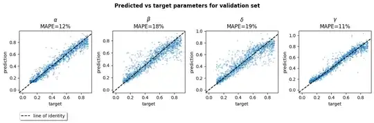
Using an LSTM, I get 10-20% prediction error across the four parameters. I trained it on a relatively wide range of parameter and initial values, and would expect performance to be better if you restrict the range. You could also tune the model further and/or train for longer.
Model size: 2304 trainable parameters
epoch  1/100  [TRN loss:  0.213 | mape [54 56 55 57]] [VAL loss:  0.210 | mape [57 55 55 54]]
...
epoch 100/100 [TRN loss:  0.023 | mape [12 17 17 11]] [VAL loss:  0.025 | mape [12 18 19 11]]
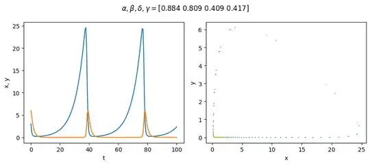
I sample parameter sets randomly, where each parameter is drawn from the range [0.1, 0.9), and the initial values are also randomly selected between [1, 50). One such sample:
If you use different ranges across the parameters, it helps to use loss weighting in order to give the smaller parameters a chance to improve (you could alternatively normalise the targets to get them on the same scale).
I first use SciPy's solve_ivp() to solve for the $x(t), y(t)$ trajectories. Then I train a one-layer LSTM to reduce the MSE between the predictions and the targets. I enforce positive values for each parameter using a Softplus() layer.
The training dataset comprised around 3800 sequences, where each sequence covered the time-span (0, 100) in 200 steps. Other training hyperparameters were: batch size of 64, 100 epochs, single-layer LSTM with a hidden size of 64, and the NAdam optimizer.
I tracked the MAPE for each parameter. It seems like $\beta$ and $\delta$ were harder to get right because their MAPEs were closer to 20%, whereas the $\alpha$ and $\gamma$ parameters were around 10%. The final validation loss was 0.025.
Reproducible example
Synthesise data and split:
import numpy as np
from matplotlib import pyplot as plt
from scipy.integrate import solve_ivp
np.random.seed(0)

Data for testing

n_sequences = 5_000
n_timesteps = 200
t_span = (0, 100)
alpha_span = (0.1, 0.9)
beta_span = (0.1, 0.9)
delta_span = (0.1, 0.9)
gamma_span = (0.1, 0.9)
x0_span = (1, 50)
y0_span = (1, 50)
#Sample n_sequences parameter sets from above parameters
alphas, betas, deltas, gammas = [
    np.random.uniform(*span, size=n_sequences)
    for span in [alpha_span, beta_span, delta_span, gamma_span]
]
parameters = np.column_stack([alphas, betas, deltas, gammas])
initial_values = np.column_stack([
    np.random.randint(x0_span, size=n_sequences),
    np.random.randint(y0_span, size=n_sequences)
])

Solve for the x/y trajectories of each set of parameters

def solve_lotka_volterra(parameters, xy0, t_span, n_timesteps):
    def lokta_volterra(t, xy, alpha, beta, delta, gamma):
        x, y = xy.T
    dx_dt = alpha*x - beta*x*y
    dy_dt = delta*x*y - gamma*y
    return np.column_stack([dx_dt, dy_dt])
#\def lotka_voleterra

t_eval = np.linspace(*t_span, num=n_timesteps)
t_span = t_eval.min(), t_eval.max()

solver_results = solve_ivp(
    lokta_volterra, t_span, xy0, t_eval=t_eval, args=parameters
)

if not solver_results['success']:
    print('[!] solve_ivp failed |', solver_results['message'])

return solver_results['y'].T #returns (n_timesteps, 2)


#For each parameter set, solve for the trajectory shaped (n_timesteps, 2)
Stack to (n_sequences, n_timesteps, 2)
sequences = np.stack(
    [solve_lotka_volterra(params_i, xy0_i, t_span, n_timesteps)
     for params_i, xy0_i in zip(parameters, initial_values)
     ],
     axis=0
)

Train-validation split

from sklearn.model_selection import train_test_split
splits = train_test_split(sequences, parameters, train_size=3/4)
sequences_trn, sequences_val, parameters_trn, parameters_val = splits
Visualise a randomly-selected sample:
#
#Visualise a random sample from train-val set
#
ix = np.random.randint(n_sequences)
x, y = sequences[ix].T
params = parameters[ix]
x, y = sequences[np.random.randint(n_sequences)].T
t = np.linspace(*t_span, n_timesteps)
plt.suptitle(r'$\alpha, \beta, \delta, \gamma=$' + str(params.round(3)))
plt.subplot(121)
plt.plot(t, x, t, y)
plt.xlabel('t')
plt.ylabel('x, y')
plt.subplot(122)
plt.scatter(x, y, marker='.', c=t, s=8, edgecolors='none')
plt.xlabel('x')
plt.ylabel('y')
plt.gcf().set_size_inches(9, 4)
plt.tight_layout()
To PyTorch tensors, and wrap in a batch loader:
import torch
from torch import nn
from torch.utils.data import TensorDataset, DataLoader
n_features = sequences.shape[-1] #x, y
output_size = parameters.shape[1] #alpha, beta, delta, gamma

Scale dataset

from sklearn.preprocessing import StandardScaler, MinMaxScaler
scaler = StandardScaler().fit(sequences_trn.reshape(-1, n_features))
X_trn = scaler.transform(sequences_trn.reshape(-1, n_features)).reshape(sequences_trn.shape)
X_val = scaler.transform(sequences_val.reshape(-1, n_features)).reshape(sequences_val.shape)

To tensor dataset

trn_dataset = TensorDataset(torch.tensor(X_trn).float(), torch.tensor(parameters_trn).float())
val_dataset = TensorDataset(torch.tensor(X_val).float(), torch.tensor(parameters_val).float())
#Batchify
batch_size = 64
trn_loader = DataLoader(trn_dataset, batch_size=batch_size, shuffle=True)
val_loader = DataLoader(val_dataset, batch_size=batch_size)
Define and train a model, reporting progress:
torch.manual_seed(0)
np.random.seed(0)
class LambdaLayer (nn.Module):
    def init(self, func):
        super().init()
        self.func = func
def forward(self, x):
    return self.func(x)


model = nn.Sequential(
    #B L C
nn.LSTM(input_size=n_features, hidden_size=64, num_layers=1, batch_first=True, proj_size=output_size),
#output: B L D*out, h_n: D*layers B out, c_n: D*layers B cell

LambdaLayer(lambda output_hncn: output_hncn[0][:, -1]),

#Params must be positive
nn.Softplus(),

)
print(
    'Model size:',
    sum(p.numel() for p in model.parameters() if p.requires_grad),
    'trainable parameters'
)
optimizer = torch.optim.NAdam(model.parameters())
n_epochs = 100
#Balance losses wrt largest target
target_weights = torch.tensor(
    parameters_trn.mean(axis=0).max() / parameters_trn.mean(axis=0)
).float().ravel()
target_weights = torch.tensor([1, 1, 1, 1]) #no balancing
@torch.no_grad()
def calc_metrics(model, loader, target_weights=None):
    model.eval()
if target_weights is None:
    target_weights =  torch.ones(output_size)

cum_loss = 0
maes = []
mapes = []

for X_mb, target_mb in loader:
    preds = model(X_mb)
    cum_loss += preds.sub(target_mb).pow(2).mul(target_weights).sum()

    mae_pertarget = preds.sub(target_mb).abs().mean(dim=0)
    mape_pertarget = mae_pertarget.div(target_mb).mul(100)

    maes.append(mae_pertarget)
    mapes.append(mape_pertarget)

loss = cum_loss / len(loader.dataset)
maes = np.row_stack(maes)
mapes = np.row_stack(mapes)

return loss, maes.mean(axis=0), mapes.mean(axis=0)


Training loop

for epoch in range(n_epochs):
    model.train()
for (X_mb, target_mb) in trn_loader:
    preds = model(X_mb)

    loss = preds.sub(target_mb).pow(2).mul(target_weights).mean()

    optimizer.zero_grad()
    loss.backward()
    optimizer.step()
#/end of epoch

# if (epoch % 5) != 0:
#     continue
model.eval()
with torch.no_grad():
    trn_loss, _, trn_mapes = calc_metrics(model, trn_loader, target_weights)
    val_loss, _, val_mapes = calc_metrics(model, val_loader, target_weights)

    print(
        f'epoch {epoch + 1:2d}/{n_epochs}',
        f'[TRN loss: {trn_loss:6.3f} | mape {trn_mapes.round()}]',
        f'[VAL loss: {val_loss:6.3f} | mape {val_mapes.round()}]',
    )
Visualise targets and predicted values:
#
# Visualise predicted vs target parameters, for each parameter
#
model.eval()
with torch.no_grad():
    trn_preds = torch.concatenate([model(X_mb) for X_mb, _ in trn_loader], dim=0).numpy()
    val_preds = torch.concatenate([model(X_mb) for X_mb, _ in val_loader], dim=0).numpy()
trn_loss, trn_maes, trn_mapes = calc_metrics(model, trn_loader, target_weights)
val_loss, val_maes, val_mapes = calc_metrics(model, val_loader, target_weights)
viz_val = True
if viz_val:
    use_preds = val_preds
    use_mapes = val_mapes
else:
    use_preds = trn_preds
    use_mapes = trn_mapes
pred_alpha, pred_beta, pred_delta, pred_gamma = use_preds.T
f, axs = plt.subplots(ncols=output_size, figsize=(12, 3.5), layout='tight')
for ax, pred, target, name, mape in zip(
    axs,
    use_preds.T,
    parameters_val.T,
    r'$\alpha$ $\beta$ $\delta$ $\gamma$'.split(),
    use_mapes
):
    ax.scatter(target, pred, marker='.', alpha=0.3, edgecolors='none')
    ax.set_title(f'{name}\nMAPE={mape:.0f}%')
    ax.set(xlabel='target', ylabel='prediction')
    ax.axline([0, 0], slope=1, linestyle='--', color='black')
axs[0].plot([np.nan], [np.nan], linestyle='--', color='black', label='line of identity')
f.legend(loc='lower left', shadow=True, bbox_to_anchor=(0.05, -0.1))
f.suptitle(f'Predicted vs target parameters for {"validation" if viz_val else "train"} set', weight='bold');

