It seems like recall is low for class 2, leading to a lower $F_1$ score. You are tuning using AUC, but I think you are looking for good $F_1$ performance, so I would suggest tuning for $F_1$ instead.
I tuned a HistGradientBoostingClassifier under CV, using f1_macro as the scoring metric. f1_macro helps select for a model that has good class-averaged precision-recall balance (averaging $F_1^{class~1}, F_1^{class~2}, F_1^{class~3}$).
After tuning the model, I get improved class 2 performance whilst retaining good class 1 and class 3 scores:
Validation set:
              precision    recall  f1-score   support
     1.0       0.99      0.96      0.97       480
     2.0       0.79      0.90      0.84        71
     3.0       0.95      1.00      0.97        52

accuracy                           0.96       603

macro avg       0.91      0.95      0.93       603
weighted avg       0.96      0.96      0.96       603
Example
Using OP's linked fetal_health.csv.
Load data and split off a test set:
import pandas as pd
import numpy as np
from matplotlib import pyplot as plt
from sklearn.model_selection import train_test_split
#Load data
df = pd.read_csv('fetal_health.csv')
#Split off a test set (not used further)
df_cv, df_test = train_test_split(df, test_size=0.15, random_state=0, stratify=df.fetal_health)
#Glimpse a random sample of data
features_df, labels_ser = df_cv.drop(columns='fetal_health'), df_cv.fetal_health
features_df.sample(frac=1.0).iloc[:10].T.style.set_caption(f'(%d samples, %d features)' % features_df.shape)
Randomized search for hyperparameters that optimize f1_macro:
from sklearn.ensemble import HistGradientBoostingClassifier
from sklearn.base import clone
from sklearn.model_selection import RandomizedSearchCV
from scipy.stats import randint, loguniform
np.random.seed(0)
param_grid = {
    'learning_rate': loguniform(1e-3, 1),
    'max_leaf_nodes': randint(2, 31),
    'max_depth': randint(2, 9),
    'min_samples_leaf': randint(1, 100),
    'l2_regularization': loguniform(1e-3, 100),
    'class_weight': ['balanced', None]
}
hgb = HistGradientBoostingClassifier(scoring='f1_macro', validation_fraction=0.2)
tuner = RandomizedSearchCV(
    hgb, param_grid,
    n_iter=300,
    cv=5,
    scoring='f1_macro',
    n_jobs=-1
).fit(features_df, labels_ser)
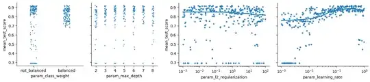
Display CV results as table and graph, select the final hyperparemeters, and report detailed performance using classification_report:
results_df = (
    pd.DataFrame(tuner.cv_results_)
    .sort_values('mean_test_score', ascending=False)
    .replace({None: 'not_balanced'})
    .reset_index(drop=True)
    .loc[:, lambda df_: ~df_.columns.isin( df_.filter(like='split').columns )]
    .loc[:, lambda df_: ~df_.columns.isin( df_.filter(like='time').columns )]
    .drop(columns=['params', 'rank_test_score'])
    .pipe(lambda df_: display(df_) or df_)
)
#results_df = results_df.loc[results_df.mean_test_score > 0.8]
import seaborn as sns
g = sns.PairGrid(
    results_df, y_vars='mean_test_score',
    x_vars=['param_class_weight', 'param_max_depth'],
    aspect=1, height=3
)
g.map(sns.stripplot, marker='.', alpha=0.8)
plt.show()
g = sns.PairGrid(
    results_df, y_vars='mean_test_score',
    x_vars=['param_l2_regularization', 'param_learning_rate'],
    aspect=1.3, height=3
)
g.map(sns.regplot, lowess=True, marker='.')
[ax.set(xscale='log') for ax in g.axes.ravel()]
plt.show()
g = sns.PairGrid(
    results_df, y_vars='mean_test_score',
    x_vars=['param_max_leaf_nodes', 'param_min_samples_leaf'],
    aspect=1, height=4
)
g.map(sns.regplot, lowess=True, marker='.')

#Selected parameters

tuned_params = {
    k.replace('param_', ''): v for k, v in
    results_df.iloc[1].filter(like='param').to_dict().items()
}
display('Selected hyperparams:', tuned_params)

#Fit a model to assess its classification report

from sklearn.metrics import classification_report
trn_ixs, val_ixs = train_test_split(range(len(features_df)), test_size=1/3, random_state=0)
xgb_tuned = clone(hgb).set_params(**tuned_params)
print(classification_report(
    y_true=labels_ser.iloc[val_ixs],
    y_pred=
    clone(xgb_tuned)
    .fit(features_df.iloc[trn_ixs], labels_ser.iloc[trn_ixs])
    .predict(features_df.iloc[val_ixs])
))
Selected hyperparams:
{'class_weight': 'balanced',
 'l2_regularization': 0.9209225155490897,
 'learning_rate': 0.34103365984137557,
 'max_depth': 5,
 'max_leaf_nodes': 5,
 'min_samples_leaf': 10}
Final metrics reported on test set:
#Final measure on the test set
if False:
    print(classification_report(
        y_true=df_test['fetal_health'],
        y_pred=
        clone(xgb_tuned)
        .fit(features_df, labels_ser)
        .predict(df_test.drop(columns='fetal_health'))
    ))
Some feature visualisation for interest:
from scipy.spatial.distance import squareform
from scipy.cluster import hierarchy
feature_correlations = features_df.corr(method='spearman').to_numpy()
np.fill_diagonal(
    feature_distances := 1 - np.abs(feature_correlations + feature_correlations.T) / 2,
    0
)
linkage = hierarchy.linkage(squareform(feature_distances), method='single')
cut_threshold = 0.4
f, ax = plt.subplots(figsize=(12, 4.5), layout='tight')
dendrogram = hierarchy.dendrogram(
    linkage,
    color_threshold=cut_threshold,
    labels=features_df.columns,
    leaf_font_size=8,
    orientation='right', ax=ax
)
ax.set_yticklabels(ax.get_yticklabels(), fontweight='bold')
ax.spines[['top', 'right']].set_visible(False)
ax.axvline(cut_threshold, linewidth=6, alpha=0.2, color='blue')
ax.axvline(cut_threshold, linewidth=3, alpha=0.2, color='red')
ax.set_xlabel('linkage distance')
plt.show()
#CCC stats
cophenetic = hierarchy.cophenet(linkage, squareform(feature_distances))
print('cophenetic correlation coefficient:', cophenetic[0])
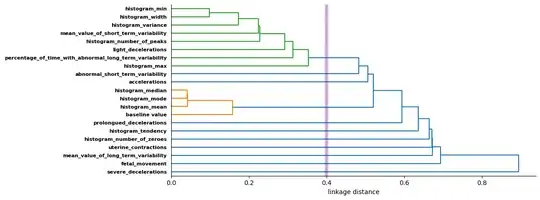
cophenetic correlation coefficient: 0.84
Simplified code
import pandas as pd
import numpy as np
from matplotlib import pyplot as plt
import seaborn as sns
from sklearn.metrics import classification_report
from sklearn.model_selection import train_test_split
from sklearn.ensemble import HistGradientBoostingClassifier
from sklearn.model_selection import RandomizedSearchCV
np.random.seed(0)

Load and split off a test set

#Load data
df = pd.read_csv('fetal_health.csv')
#Split off a test set (not used further)
df_cv, df_test = train_test_split(df, test_size=0.15, random_state=0, stratify=df.fetal_health)
#Separate features and labels
features_df, labels_ser = df_cv.drop(columns='fetal_health'), df_cv.fetal_health
features_df.head()

Randomized search for hyperparameters that maximise f1_macro

param_grid = {
    'learning_rate': np.logspace(-3, 0, num=1000), #values 10^-3 to 10^0
    'max_leaf_nodes': np.random.randint(2, 31, size=1000),
    'max_depth': np.random.randint(2, 9, size=1000),
    'min_samples_leaf': np.random.randint(1, 100, size=1000),
    'l2_regularization': np.logspace(-3, 2, num=1000), #values 10^-3 to 10^2
    'class_weight': ['balanced', None]
}
hgb = HistGradientBoostingClassifier(scoring='f1_macro', validation_fraction=0.2)
tuner = RandomizedSearchCV(hgb, param_grid, n_iter=100, cv=5, scoring='f1_macro')
tuner.fit(features_df, labels_ser)

Display CV results as table and graph, select the final hyperparemeters,
and report detailed performance using classification_report:

results_df = (
    pd.DataFrame(tuner.cv_results_)
    .sort_values('rank_test_score')
    .replace({None: 'not_balanced'})
)
display(results_df)

Plot score vs parameter values, for different parameters

#Score vs class_weight, and score vs max_depth
g = sns.PairGrid(
    results_df,y_vars='mean_test_score',
    x_vars=['param_class_weight', 'param_max_depth']
)
g.map(sns.stripplot)
plt.show()
#Score vs l2_regularisation, and score vs learning_rate
g = sns.PairGrid(
    results_df, y_vars='mean_test_score',
    x_vars=['param_l2_regularization', 'param_learning_rate'],
)
g.map(sns.regplot, lowess=True)
plt.show()
#Score vs max_leaf_nodes, and score vs min_samples_leaf
g = sns.PairGrid(
    results_df, y_vars='mean_test_score',
    x_vars=['param_max_leaf_nodes', 'param_min_samples_leaf'],
)
g.map(sns.regplot, lowess=True)

#Selected hyperparameters for model

hgb_tuned = HistGradientBoostingClassifier(
    scoring='f1_macro',
    validation_fraction=0.2,
#Selected from tuning:
class_weight='balanced',
l2_regularization=0.9,
learning_rate=0.3,
max_depth=5,
max_leaf_nodes=5,
min_samples_leaf=10,

)

#Fit a model to assess its classification report

features_trn, features_val, labels_trn, labels_val = train_test_split(features_df, labels_ser, test_size=1/3)
hgb_tuned.fit(features_trn, labels_trn)
predictions = hgb_tuned.predict(features_val)
clf_report = classification_report(y_true=labels_val, y_pred=predictions)
print(clf_report)

#Final measure on the test set

if False:
    #Start by fitting on all the non-test data
    hgb_tuned.fit(features_df, labels_ser)
features_test = df_test.drop(columns='fetal_health')
test_predictions = hgb_tuned.predict(features_test)

clf_report = classification_report(y_true=df_test['fetal_health'], y_pred=test_predictions)
print(classification_report(clf_report))

