4

I have a dataset of measurements $Y$ to which I want to fit a custom distribution, and thereby obtain an estimate of the distribution's parameters.

enter image description here

Based on domain knowledge, I know that the process generating $Y$ is a weighted mixture of two Gamma distributions:

$Y\sim w\times\Gamma(\alpha_1, \theta_1)+(1-w)\times\Gamma(\alpha_2, \theta_2)$

I want to estimate $w$, $\alpha_1$, $\theta_1$, $\alpha_2$, and $\theta_2$.

SciPy has various standard distributions but I want a more general way to specify my custom mixture.

scipy.optimize.curve_fit doesn't quite fit the bill because I want to estimate the distribution from the data rather than directly fit a curve.

How can this be done using SciPy?

3 Answers3

6

Start by defining a function that constructs the PDF model. In your case it's a mixture of two Gamma distributions, but it could be anything else:

def two_gamma(y_samples, w, alpha1, scale1, alpha2, scale2):
    #Construct the current estimated PDF
    gamma1_pdf = stats.gamma.pdf(y_samples, alpha1, scale=scale1)
    gamma2_pdf = stats.gamma.pdf(y_samples, alpha2, scale=scale2)
    y_pdf_estimate = w * gamma1_pdf + (1 - w) * gamma2_pdf
return y_pdf_estimate

You can then use scipy.optimize.minimize to tune the parameters such that the negative log-likelihood (NLL) is minimized. The function two_gamma_mle below uses the estimated parameters to construct a PDF, and then returns a score (NLL) of how well the parameters match the data:

def two_gamma_mle(params):
    #Construct the current estimated PDF (at the data points Y)
    y_pdf_estimate = two_gamma(Y, *params)
#Return the sample-averaged negative log likelihood
avg_neg_ll = -np.log(y_pdf_estimate + 1e-8).mean()
return avg_neg_ll

results = optimize.minimize(
  two_gamma_mle,
  x0=initial_guess,
  bounds=bounds
)

w, alpha1, scale1, alpha2, scale2 = results['x']

You could technically use curve_fit to fit the mixture model to a kernel density estimate of $Y$, but the MLE approach above is more direct and works better.

Also, see this informative question that neatly encapsulates things for an arbitrary number of components.

Demo

Consider the test dataset below. We have the samples $Y$, and want to estimate the parameters of the $\Gamma$ mixture (green) that generated it.

enter image description here

Using minimize() results in a good fit$^\dagger$ to the reference distribution:

Converged? True
Estimated params: [ 0.49 19.81  0.51  2.03  0.98]

enter image description here

Tips for resolving numerical issues

Some suggestions that help with preventing non-convergence and overflow:

  • Return the average NLL rather than the sum, to reduce the chance of overflow when there are lots of samples

  • Add a small value $\epsilon=1\times10^{-8}$ before taking the $log$: np.log(... + epsilon). Too small and it's ineffective; too large and it distorts the optimization too much.

  • Break symmetry - don't initialise parameters to identical values (add a bit of uniform noise, for example).

  • If a parameter ought to be bounded $(0, 1)$, non-negative, etc, supply the bounds= parameter.

  • You can also try all the method= options. When a fit is failing, you may find some methods do a better job than others.

Code

Imports, data for testing, and visualisation:

import numpy as np
from scipy import stats

import matplotlib.pyplot as plt

#Sample a PDF using inverse transform sampling def sample_pdf(x, pdf_x, n_samples=1000): cdf = np.cumsum(pdf_x / pdf_x.sum())

cdf_vals_sampled = np.random.uniform(0, 1, n_samples)
cdf_ixs = np.searchsorted(cdf, cdf_vals_sampled)

return x[cdf_ixs]

def two_gamma(y_samples, w, alpha1, scale1, alpha2, scale2): #Construct the current estimated PDF gamma1_pdf = stats.gamma.pdf(y_samples, alpha1, scale=scale1) gamma2_pdf = stats.gamma.pdf(y_samples, alpha2, scale=scale2) y_pdf_estimate = w * gamma1_pdf + (1 - w) * gamma2_pdf

return y_pdf_estimate

Data for testing: a bimodal Y comprised of two Gamma distributions

np.random.seed(0)

W = 0.5 ALPHA1, SCALE1 = 2, 1 ALPHA2, SCALE2 = 20, 0.5

#Create PDF of Y which is a mixture of the two gamma distributions y_axis = np.linspace(0, 20, num=5_000) pdf_y = two_gamma(y_axis, W, ALPHA1, SCALE1, ALPHA2, SCALE2) #wg1 + (1-w)g2

#Sample data for testing Y = sample_pdf(y_axis, pdf_y, n_samples=5_000)

Visualise distribution of Y and its underlying components

pdf_gamma1 = stats.gamma(ALPHA1, scale=SCALE1).pdf(y_axis) pdf_gamma2 = stats.gamma(ALPHA2, scale=SCALE2).pdf(y_axis)

f, axs = plt.subplots(nrows=2, ncols=1, figsize=(8, 4), sharex=True, layout='tight')

ax = axs[0] ax.plot(y_axis, pdf_gamma1, label='$\gamma_1$') ax.plot(y_axis, pdf_gamma2, label='$\gamma_2$') ax.plot( y_axis, pdf_y, label='Y ~ $w\gamma_1 + (1 - w)\gamma_2$', linewidth=7, color='green', alpha=0.25 )

ax.legend(ncols=3, shadow=True) ax.set(ylabel='PDF', title='PDFs')

ax.spines[['top', 'right']].set_visible(False) ax.spines.bottom.set_bounds(0, 20) ax.spines.left.set_bounds(0, 0.2)

Visualise data points

ax = axs[1] ax.plot(Y, range(len(Y)), linestyle='none', marker='.', markersize=1, alpha=0.8, color='black')

ax.set(xlabel='y', ylabel='sample index', title='Samples')

ax.spines[['top', 'right']].set_visible(False) ax.spines.bottom.set_bounds(0, 20) ax.spines.left.set_bounds(0, 4000)

Fit to the data and report results:

from scipy import optimize

def two_gamma_mle(params): #Construct the current estimated PDF (at the data points Y) y_pdf_estimate = two_gamma(Y, *params)

#Return the sample-averaged negative log likelihood
avg_neg_ll = -np.log(y_pdf_estimate + 1e-8).mean()
return avg_neg_ll

Fit using scipy.optimize.minimize()

initial_guess = [1] * 5 bounds = [(0, 1)] + [(0, None)] * 4 #w bounded (0, 1). Other params (0, inf).

res = optimize.minimize(two_gamma_mle, x0=initial_guess, bounds=bounds) estimated_params = (w, alpha1, scale1, alpha2, scale2) = res['x']

print('Converged?', res['success']) print('Estimated params:', estimated_params.round(2))

View results

ax = plt.figure(figsize=(8, 3), layout='tight').add_subplot()

ax.plot(y_axis, pdf_y, linewidth=3, label='target PDF')

y_pdf_fit = two_gamma(y_axis, *estimated_params) ax.plot(y_axis, y_pdf_fit, linestyle='--', color='lawngreen', label='estimated PDF') ax.legend() ax.set(xlabel='y', ylabel='PDF', title='Target and MLE-estimated PDF') ax.spines[['top', 'right']].set_visible(False) ax.spines.left.set_bounds(0, 0.15) ax.spines.bottom.set_bounds(0, 20)


$^\dagger$The estimated parameters for the individual components are swapped round compared to the ground truth, but the overall fit is good. You can constrain the parameters if required and/or specify a more precise initial guess.

5

You want to use empirical cumulative distribution fitting (ECDF). Simply generate the cumulative distribution CDF for the $Y$ data over the range of $X$ when divided into e.g. 100 equally-spaced non-overlapping bins. Then mix two $\boldsymbol{\Gamma}$ distributions together based on candidate values of parameters, and generate the CDF for that mixture of PDFs. Calculate the MSE (over the 100 bins) between observed CDF and the sumulated CDF. Employ a greedy hill climbing metaheuristic to solve for the optimum parameters which minimize MSE. It works out that CDFs are used more commonly to fit distributions because you know that the CDF values are 0 and 1 at the min(max) values of $X$.

wjktrs
  • 358
  • 5
4

This post is just a code implementation and demo of the MLE approach outlined in this answer (generalised to multiple components using this implementation by @Galen), and the empirical CDF (ECDF) fitting approach described in the answer by @wjktrs.

I encapsulate the functionality in a GammaMixture class (originally defined by @Galen). The class provides methods for running three types of fitting for mixture parameter estimation:

  • Maximum likelihood estimation

    • Minimizes the negative log-likelihood between the data and the mixture PDF
  • ECDF fitting using regular least-squares

    • Minimises the MSE between the mixture CDF and the data CDF (latter estimated using a histogram)
  • ECDF fitting using isotonic regression

    • As above, but constraining the fitted CDF to be non-decreasing (as a valid CDF should be).

I found that the MLE approach was bar far the most stable. The ECDF fitting approaches were okay up to 3 components, but convergence was less predictable for 4+ components (the least-squares variant sometimes handled 4 components, whereas isotonic regression did not).

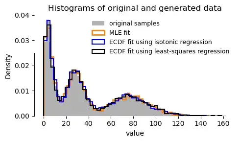
A comparison of fits using the three methods (sample data comprises 3 $\Gamma$ components):
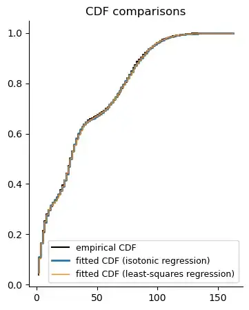
enter image description here

Fitted CDFs:

enter image description here

Reproducible example

Class for fitting and sampling a mixture of $\Gamma$ distributions (you can easily modify it to use other distributions defined in SciPy):

import numpy as np
import matplotlib.pyplot as plt

from scipy.stats import gamma from scipy.special import softmax from scipy.optimize import minimize

from typing import Tuple, Dict

class GammaMixture: def init(self, n_components: int): self.n_components = n_components self.weights = np.ones(n_components) / n_components self.alphas = np.ones(n_components) self.scales = np.ones(n_components)

    self._cdf = self._cdf_exact #alternatively: self._cdf_approx


def _pdf(self, x: np.ndarray) -> np.ndarray:
    mixture = np.row_stack([
        self.weights[i] * gamma.pdf(x, self.alphas[i], scale=self.scales[i])
        for i in range(self.n_components)
    ]).sum(axis=0)

    return mixture


def _cdf_approx(self, x: np.ndarray) -> np.ndarray:
    """CDF by normalising pre-computed PDF. Fast but approximate."""
    pdf = self._pdf(x)
    return np.cumsum(pdf / pdf.sum()) 


def _cdf_exact(self, x: np.ndarray) -> np.ndarray:
    """CDF exact values using SciPy"""
    mixture_cdf = np.row_stack([
        self.weights[i] * gamma.cdf(x, self.alphas[i], scale=self.scales[i])
        for i in range(self.n_components)
    ]).sum(axis=0)

    return mixture_cdf


def _get_initial_guesses_and_bounds(self) -> Dict[str, np.ndarray]:
    initial_params = np.concatenate([
        np.log(self.weights),
        np.ones(2 * self.n_components) + np.random.uniform(0, 0.01, 2*self.n_components) #break symmetry
    ])
    bounds = [(None, None)]*self.n_components + [(0, None)] * (2*self.n_components)
    return {'x0': initial_params, 'bounds': bounds}


def _set_weights_alphas_scales(self, params: np.ndarray) -> None:
    #Write mininmizer's results['x'] into self's weights, alphas, and scales
    logits, self.alphas, self.scales = np.split(params, [self.n_components, 2*self.n_components])
    self.weights = softmax(logits)


def _cdf_mse(self, params: np.ndarray, data: np.ndarray, n_bins: int) -> float:
    #Compute data's ECDF. Could alternatively precompute once in calling function.
    hist, bin_edges = np.histogram(data, bins=n_bins)
    empirical_cdf = np.cumsum(hist / hist.sum())

    #Candidate CDF
    self._set_weights_alphas_scales(params)        
    candidate_cdf = self._cdf(bin_edges[1:])

    cdf_sse = ((candidate_cdf - empirical_cdf)**2).sum()
    return cdf_sse


def fit_using_ecdf(self, data: np.ndarray, n_bins: int = 100, enforce_monotonicity: bool = False) -> Tuple[np.ndarray, np.ndarray, np.ndarray]:
    def _constraints_fun(params):
        self._set_weights_alphas_scales(params)
        _, bin_edges = np.histogram(data, bins=n_bins)
        cdf = self._cdf(bin_edges)
        return np.diff(cdf)

    result = minimize(
       fun=self._cdf_mse,
       args=(data, n_bins),
       **self._get_initial_guesses_and_bounds(),
       constraints={'type': 'ineq', 'fun': _constraints_fun} if enforce_monotonicity else (),
    )
    print(
        'Success?', result['success'],
        '\n CDF MSE:', result['fun'],
        '\n NLL:    ', self._negative_log_likelihood(result['x'], data),
        '\n nit:    ', result['nit'],
        end='\n\n'
    )

    self._set_weights_alphas_scales(result['x'])
    return self.weights, self.alphas, self.scales


def _negative_log_likelihood(self, params: np.ndarray, data: np.ndarray) -> float:
    self._set_weights_alphas_scales(params)

    eps = 1e-8
    neg_log_likelihood = -np.log(self._pdf(data) + eps).mean()
    return neg_log_likelihood

def fit_using_mle(self, data: np.ndarray) -> Tuple[np.ndarray, np.ndarray, np.ndarray]:
    result = minimize(
        fun=self._negative_log_likelihood,
        args=(data,),
        **self._get_initial_guesses_and_bounds(),
    )
    print(
        'Success?', result['success'],
        '\n NLL:', result['fun'],
        '\n nit:', result['nit'],
        end='\n\n'
    )

    self._set_weights_alphas_scales(result['x'])
    return self.weights, self.alphas, self.scales

def sample(self, n_samples: int) -> np.ndarray:
    components = np.random.choice(self.n_components, size=n_samples, p=self.weights)
    samples = np.array([gamma.rvs(self.alphas[i], scale=self.scales[i]) for i in components])
    return samples

Compare the various fitting methods:

# np.random.seed(10)
n_per_component = 2_000
data = np.concatenate([
    gamma.rvs(a=2.0, scale=3, size=n_per_component),
    gamma.rvs(a=15.0, scale=2., size=n_per_component),
    gamma.rvs(a=20.0, scale=4., size=n_per_component),
    # gamma.rvs(a=55.0, scale=3., size=n_per_component),
])

n_components = 3

MLE fit

gamma_mixture = GammaMixture(n_components) gamma_mixture.fit_using_mle(data) samples_mle = gamma_mixture.sample(n_samples=len(data))

ECDF fits

gamma_mixture = GammaMixture(n_components) gamma_mixture.fit_using_ecdf(data, n_bins=100, enforce_monotonicity=True) samples_ecdf_isotonic = gamma_mixture.sample(n_samples=len(data))

gamma_mixture = GammaMixture(n_components) gamma_mixture.fit_using_ecdf(data, n_bins=100, enforce_monotonicity=False) samples_ecdf_mse = gamma_mixture.sample(n_samples=len(data))

Visualise results

f, ax = plt.subplots(figsize=(5, 3), layout='tight')

Histogram of original data

ax.hist( data, bins=70, density=True, color='black', alpha=0.3, label='original samples' )

Histogram of new samples from MLE fit

ax.hist( samples_mle, bins=50, density=True, histtype='step', color='tab:orange', linewidth=2, label='MLE fit' )

Histogram of new samples from CDF fit

ax.hist( samples_ecdf_isotonic, bins=50, density=True, histtype='step', color='blue', linewidth=1.5, label='ECDF fit using isotonic regression' )

ax.hist( samples_ecdf_mse, bins=50, density=True, histtype='step', color='black', linewidth=1.5, label='ECDF fit using least-squares regression' )

#Formatting ax.set(xlabel='value', ylabel='Density', title='Histograms of original and generated data') ax.legend(fontsize=9, framealpha=0)

ax.spines[['top', 'right', 'bottom']].set_visible(False) ax.spines.left.set_bounds(0, 0.025)

For ECDF fitting methods, compare the fitted CDFs:

counts, bin_edges = np.histogram(data, bins=100, density=True)
empirical_cdf = np.cumsum(counts / counts.sum())
plt.step(bin_edges[1:], empirical_cdf, color='black', label='empirical CDF')

gamma_mixture = GammaMixture(n_components) gamma_mixture.fit_using_ecdf(data, n_bins=100, enforce_monotonicity=True) fitted_cdf = gamma_mixture._cdf(bin_edges[1:]) plt.step(bin_edges[1:], fitted_cdf, linewidth=2, label='fitted CDF (isotonic regression)')

gamma_mixture = GammaMixture(n_components) gamma_mixture.fit_using_ecdf(data, n_bins=100, enforce_monotonicity=False) fitted_cdf = gamma_mixture._cdf(bin_edges[1:]) plt.step(bin_edges[1:], fitted_cdf, linewidth=1, label='fitted CDF (least-squares regression)')

plt.title('CDF comparisons') plt.legend(fontsize=9) plt.gcf().set_size_inches(4, 5) plt.gca().spines[['right', 'top']].set_visible(False)