0

I am trying to build a model to estimate the ATE of Campaign B (B1) on CTR (Click-thru-Rate), with Campaign A as the baseline (B0), represented by column 'a_or_b'.

Other exogenous variables are: 'nth_day' (number of days elapsed for given campaign on a given day), 'platform_Meta', 'platform_StackAdapt' (both are binary, dummy variables with 'platform_Google' being represented in the baseline.

I'm a data science graduate student, and I have taken a causal inference course, however it mostly discussed the usage of OLS. It was very clear that OLS would not work well after an attempt.

After realizing that I was better off with a model that was bound by [0, 1] (100% is the max CTR possible), I figured I'd try my hand at a Beta Regression model using statsmodels.othermod.betareg.BetaModel.

Just for reference, here is the distribution of CTR. This is the result from df.describe() for more context about the data.

It's very skewed to the right, with most values being very small (but not 0).

I'm having a difficult time determining which model (if any of them) I've created is providing a decent enough fit for me to trust the coefficient and p-val of 'a_and_b'.

From what I understand, the lower AIC for Model 3 means it is better fit, however its QQ Plot and Residuals vs Fitted look very wonky and I don't trust the results.

The results from statsmodels for both models are here.

Model 2: QQ Plot, Residuals vs Fitted

Model 3: QQ Plot, Residuals vs Fitted

I'm looking for some insights and direction regarding where to take this. Feel free to also tell me if I am completely off track . I'm here to learn!
J_H
  • 1,233
  • 9
  • 12

1 Answers1

1

Welcome to SE

I don't usually look at the summary outputs you have presented, so cannot tell you if it looks right or wrong. Instead, I find it simpler to go back to hypothesis and then use brute-force.

You mentioned p-values. So I guess you must have a null-hypothesis. I will also guess that null-hypothesis is that data is from beta-distribution (with the regression added in). So why not:

  1. Take the coefficients that your fitting gives you
  2. Generate random dependent variable with the beta-regression model that you are trying to fit
  3. Get log-likelihood for the generated data under that model
  4. Repeat until you get a distribution of log-likelihood

Now compare the log-likelihood of your data under the model, to the log-likelihood distribution. That will allow you to assess how well the model fits the data.

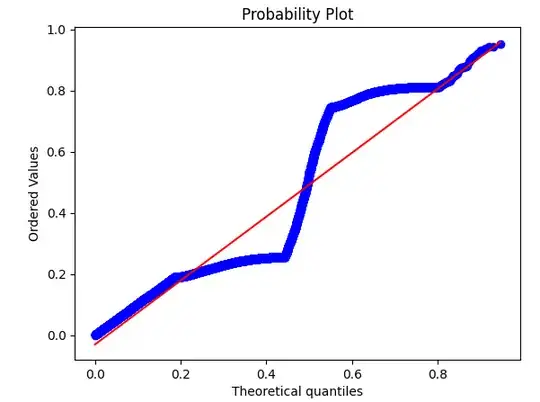
Having said that, looking at your QQ-plots, the fit does seem to be quite bad in both cases. I almost want to 'stretch' your sample quantiles so that they would fit the theoretical quantiles. This may work, I would try to come up with a function that maps your dependent variable into some another variable, also with the range $[0,1]$, but which also can model that kink you see in your qq-plots. Then fit the coefficients of that function, preferably at the same time as beta-regression (it is all max likelihood anyway).

Below is an example of a transformation that creates a somewhat similar-looking kink in qq:

import scipy as sp
import scipy.stats as sp_st
import scipy.special as sp_sp

import numpy as np import numpy.random as npr

import matplotlib as mpl import matplotlib.pyplot as pp import matplotlib.cm as cm

x = npr.beta(1.2, 3.4, size=(10000,)) lx = sp_sp.logit(x) mod_x = sp_sp.expit( lx (1.0+5.0np.exp(-((lx)2)/(0.52))) )

(osm, osr), _ = sp_st.probplot(mod_x, dist=sp_st.beta(1.2, 3.4), plot=pp)

enter image description here

Cryo
  • 563
  • 2
  • 9