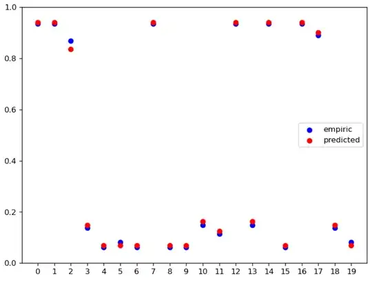
XGB predict_proba estimates don't match sum of leaves

Question

When using an XGB model in the context of binary classification, I observed that the test estimates given by predict_proba were close but not equal to the results I obtained by summing the outputs of the corresponding leaves for each observation and then converting that sum (which is a log-odds) to probability using the logistic function $\frac{e^x}{1+e^x}$. Why does this happen? What am I not taking into account and how can I recreate the results of predict_proba with the individual outputs from the trees?

My code (based on the example given in the XGB docs page) starts by fitting the model:

from sklearn.datasets import load_iris
from xgboost import XGBClassifier
from sklearn.model_selection import train_test_split
data = load_iris()
X_train, X_test, y_train, y_test = train_test_split(data['data'][data['target']!=2], 
data['target'][data['target']!=2], test_size=.2, random_state=42)
# create model instance
bst = XGBClassifier(n_estimators=5, max_depth=2, learning_rate=0.5, 
objective='binary:logistic', colsample_bytree=0.3)
# fit model
bst.fit(X_train, y_train)

After doing this I was able to retreive the individual trees of the model and hard-code them into a function to obtain the tree outputs in an array:

def empiric_model(X):
    # t0,...,t4 is for the trees and f0, f1, f2 are the features
    t0 = -0.952112317 if (X['f2']<3).all() else 0.869410515
    t1 = -0.462368667 if (X['f0']<5.5).all() else 0.51116854
    t2 = -0.571811914 if (X['f2']<3).all() else 0.569128871
    t3 = 0.403415382 if (X['f1']<3).all() else 0.0914318636 if ((3<=X['f1'])&(X['f1']<3.0999999)).all() else -0.11495477 if ((3.0999999<=X['f1'])&(X['f1']<3.4000001)).all() else -0.417713255
    t4 = 0.318558067 if (X['f1']<3).all() else 0.0555250905 if ((3<=X['f1'])&(X['f1']<3.20000005)).all() else -0.309806734
    return np.array([t0, t1, t2, t3, t4])

Then I compared both bst.predict_proba(X_test)[:,1] and the sum of the leaves outputs converted into probability. The results of that comparison are shown in the next graph:

# sum of leaf-outputs for each test observation
empirics = np.array([empiric_model(pd.DataFrame(X_test[i:i+1,:], columns=['f0','f1','f2','f3'])).sum() for i in np.arange(X_test.shape[0])])
# convert that into proba using the logistic function
empiric_probas = np.exp(empirics)/(1+np.exp(empirics))
predicted_probas = bst.predict_proba(X_test)[:,1]
plt.scatter(x=np.arange(empiric_probas.size), y=empiric_probas, c='b', label='empiric')
plt.scatter(x=np.arange(empiric_probas.size), y=predicted_probas, c='r', label='predicted')
plt.xticks(np.arange(empirico_probas.size))
plt.yticks(np.arange(0,1.1,0.2))
plt.legend(loc='center right')

I'll explicitly show these values: empiric_probas is:

array([0.9353348 , 0.9353348 , 0.86878725, 0.13712985, 0.06216319,
   0.08233362, 0.06216319, 0.9353348 , 0.06216319, 0.06216319,
   0.14927792, 0.11448531, 0.9353348 , 0.14927792, 0.9353348 ,
   0.06216319, 0.9353348 , 0.8905786 , 0.13712985, 0.08233362])

while predicted_probas is:

array([0.9411262 , 0.9411262 , 0.8354762 , 0.1493973 , 0.06825472,
   0.06825472, 0.06825472, 0.9411262 , 0.06825472, 0.06825472,
   0.16242756, 0.12502052, 0.9411262 , 0.16242756, 0.9411262 ,
   0.06825472, 0.9411262 , 0.89994967, 0.1493973 , 0.06825472])

Which as you can see are similar but not equal.

score 2 · Answer 1 · answered Apr 15 '24 at 21:19

When you call predict_proba in XGBoost, it returns the probability estimates calculated by averaging the predictions of all the individual trees in the ensemble. This averaging process considers various factors such as regularization parameters and the learning rate used during training.

The difference you're observing is because the manual calculation doesn't fully replicate the internal workings of predict_proba in XGBoost. To achieve exact alignment, you would need to mimic the averaging mechanism used in predict_proba, which might require more intricate knowledge of XGBoost's implementation details.

One option is to convert your estimator into an if-else script. The following post shows how to achieve that.

Hope it helps!

XGB predict_proba estimates don't match sum of leaves

1 Answers1